超导Tc公式与网格比较
Quantum ESPRESSO · Al 双致密网格 Tc 估算对照
目录
完整α²F及谱矩 · Al双网格计算链 · Allen–Dynes原论文
λ 与频率尺度怎样共同决定 Tc
总λ告诉我们电子与声子耦合有多强,ωlog给出按配对权重平均的振动频率尺度。声子软化可能把谱权重移到低频、增大λ,同时降低ωlog;Tc最终由两种变化共同决定。Ba₂N的应变比较正是这一例子:论文图5中4%拉伸使λ从0.59增至1.49,ωlog下降,而所采用公式的Tc从3.4升至10.8 K。机制还要返回图3、6的模式与谱峰,不能只把温度上升归为DOS增加。Qiu等,PRB105,165101。
经验公式还需要有效库仑赝势μ*。它是模型输入,并非当前DFT自动计算的物性。本页从同一谱的简式与完整公式讲起,再用Al32³、48³两条独立链的Tc(σ)检查数值差异。
先知道自己代入的是哪个公式
这次 QE 7.5 的 lambda.x 使用的是包含 ω_log 的简化 Allen–Dynes 表达式:
这里 ω_log 以 K 表示,算出的 Tc 也是 K。该式相当于将强耦合与谱形修正因子 f₁、f₂ 设为 1;没有求解各向异性的 Eliashberg 方程。不要把输出里的 K 再当作 THz 乘一次换算系数,也不要把论文中包含 f₁、f₂ 的结果与这行代码当成同一个计算。
源码计算 ωlog 时用内部谱积分的 λ 归一化,计算 Tc 时则取逐 q 求和的 λ;这正是输出中两种 λ 要分列保留的原因。后面另外从同一打印谱提取一致的频率矩,用于完整 f₁、f₂ 对照。
μ* 是有效库仑赝势参数。本例取 0.10,是输入假设,不是这次 DFT 自动求出的物性。
自己复算第 4 行,先检查分母
用打印出来的 λ=0.374486、ωlog=343.741 K 和 μ*=0.10,就能在终端复现这一行:
maxwell@maxwell:~/tc-route/replay-lambda$ python3 -c 'import math; lam=0.374486; wlog_K=343.741; mu=0.10; d=lam-mu*(1+0.62*lam); print(f"denominator = {d:.9f}"); print(f"Tc = {wlog_K/1.2*math.exp(-1.04*(1+lam)/d):.6f} K")'
denominator = 0.251267868
Tc = 0.969046 K
这是用表格舍入数字得到的复算值;从逐 q 原件重建内部值为 0.969044 K,两者都对应原生输出的 0.969 K。分母非正、近于零或输入非有限时,新增脚本会停止公式计算,不会把一个失去适用意义的指数结果解释成材料温度。这也不能被反过来当成证明材料不超导。 分母检查看的是这条拟合表达式的输入域。对正 λ,它要求 ;本行的右边约为 0.303921。靠近这条边界时,分母很小,Tc 对输入舍入和参数选择会异常敏感。这个数只由当前 λ 和公式算出,不是材料的临界库仑相互作用,也不应据此向边界外延伸 μ* 扫描。通过分母检查后,还要按同一非负谱和适用近似解释温度。
从谱中提取二阶矩,才能计算完整 f₁、f₂
只有 λ 与 ωlog 两个数,还不能决定完整 Allen–Dynes 的谱形修正。它还需要耦合加权的均方根频率 ν̄₂,不能拿普通声子 DOS 的平均频率、另一个电子展宽的频率矩,或另一条 matdyn 路线的数据来补。
| 公式版本 | 前因子 | 本例用途 |
|---|---|---|
| 原始 McMillan | 本例没有计算 ,不拿它代替 | |
| QE 7.5 的 修正式 | , | 与原生 lambda.x 逐行复算 |
| 含 、 的 Allen–Dynes | 从同一非负谱计算完整矩后单列 |
以普通频率 ν 写,同一份谱的三个积分是:
这里的归一化 λspec 必须来自这份谱。对数使用同一固定单位,可以理解为对 ν/(1 THz) 取对数,最后恢复 THz。νlog、ν̄₂ 随后乘 h×10¹²/kB 得到 K;若写成角频率则使用 ħω/kB,不能多乘 2π。复现 QE 7.5 时沿用源码的 47.9924 K/THz,已经是 K 的打印 ωlog 不再换算。
零频点不直接除以 ν 或取对数。本例零点的谱值为零,可以从正频点积分;这不是允许删掉其他材料中的异常低频峰或实质性虚频。脚本拒绝负谱,不取绝对值、不裁零后再输出一组看似合理的 Tc。
在同一谱矩下加入 f₁、f₂
谱分析程序从32³链0.020 Ry的非负打印谱得到下面的矩。逐q加权λ与谱积分λ分列,不以matdyn负谱替换。完整Allen–Dynes的强耦合、谱形因子是原论文式(34)–(38)给出的拟合关系,仍是公式近似。
设 ,完整形式为:
两种频率都换成 K 后,r 仍无量纲。f₁ 是强耦合修正,f₂ 随谱形改变;它们仍属于拟合公式,补上以后并不等于数值求解了 Eliashberg 方程。
0.020 Ry 这列的实际中间量是:
| 量 | 数值 |
|---|---|
| 0.37454456 | |
| 343.74087 K | |
| 对应温度 | 363.33106 K |
| 0.10 | |
| 1.01206929 | |
| 1.00080168 |
三行温度必须分开读:
| 数据与公式 | Tc(K) |
|---|---|
| QE 原生定义:λqsum 与原生谱 ωlog,简式 | 0.969044 |
| 同一打印谱的 λspec、ωlog,简式 | 0.970016 |
| 同一打印谱的 λspec、ωlog、ν̄₂,乘 f₁f₂ | 0.982511 |
第一到第二行包含归一化与打印谱积分的变化,第二到第三行才是在固定同一组谱矩后加入 f₁f₂。不能把第一到第三行的全部差别都说成强耦合修正,更不能把较高的一行选作更可靠的材料预测。
固定谱后改变 μ*
固定 0.020 Ry 的谱,只改变 μ*,三种定义得到:
maxwell@maxwell:~/al/tc-route$ cat data/mu-star-scan.csv
mu_star,Tc_QE_rounded_input_K,Tc_spectrum_simple_K,Tc_spectrum_full_AD_K
0.08,1.6107226584993182,1.6120500128520705,1.6347436284357797
0.09,1.2642718580381032,1.2654176885906845,1.2824457531797715
0.1,0.969046002012425,0.970016140785092,0.9825105724541605
0.11,0.7226644078867569,0.7234674219221328,0.732398924745519
0.12,0.5220046073518098,0.5226518506188913,0.5288436032754813
0.13,0.36321819742344197,0.3637237157771725,0.3678633763712934
0.14,0.24179286792772323,0.24217311358934973,0.2448239277483174
0.15,0.1526709604922883,0.15294427830078677,0.15455599724304322
0.16,0.09043153189929327,0.0906173974670778,0.09153761243237504
这些点没有重新计算 DFT;它们是同一经验公式的假设敏感性,不是独立实验或统计置信区间。μ* 从 0.08 增到 0.16 时温度明显下降,说明结论若依赖某个选择,就需要报告采用值、范围与依据。
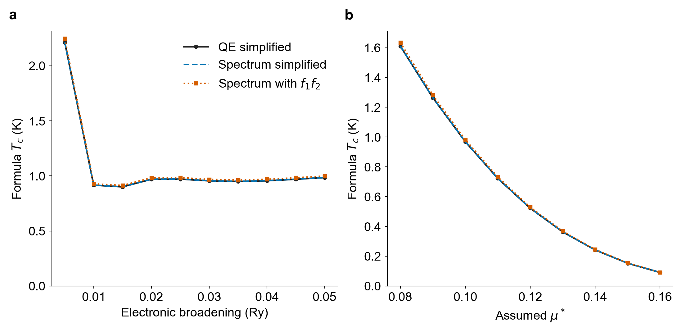
左幅保持 μ*=0.10,改变 EPC 电子展宽;右幅固定 0.020 Ry 的谱,改变 μ*。横轴回答两种不同问题。最窄展宽的离群值并不会因为乘上 f₁f₂ 就变得可信。
μ扫描与电子σ扫描分别回答模型假设和电子积分问题。两者的温度范围都不是统计置信区间。下文固定μ=0.10、相同频率谱宽与q权重,考察致密网格改变的影响。
两个目录各自跑到 lambda.x,再读两份 Tc 表
完整 EPC 会话记录了两条路径,第二条的 cp、vi、完整 Slurm 脚本及运行结果在 48³ 分支。这里直接接它们的结果,不重新写一次 SCF。
| 计算路径 | pwxall 致密 k | pwx 响应 k | 实算 q 网格 | 留给本页的原件 |
|---|---|---|---|---|
epc-q4 |
32×32×32 | 16×16×16 | 4×4×4,8 个不可约 q | 本目录的 8 个 elph.inp_lambda.*、lambda.in/out/dat |
epc-q4-k48 |
48×48×48 | 16×16×16 | 4×4×4,8 个不可约 q | 新目录独立计算的同组文件 |
两边的 pwxall 网格分别是响应网格的 2 倍、3 倍;响应网格又是 q 网格的 4 倍,所有网格均不偏移。lambda.in 使用相同的 q 权重、14 THz 谱上限、0.12 THz 频率展宽和 μ*=0.10。横轴 σ 则来自 ph.x 的十档电子积分展宽:0.005、0.010、…、0.050 Ry。这三个展宽概念要分开:SCF 占据的 degauss=0.02 Ry 没有在本图中扫描,谱函数的 0.12 THz 宽度也没有变化。
第二条链已完成 8 个 q × 3 个模式 × 10 个展宽,共 240 条模式记录。两份响应 SCF 的电荷密度文件逐字节相同,32³ 与 48³ 的致密电子数据则各自保存;第二条从头执行了两次 SCF 和所有 q 响应。原生输入、输出、核验表及本节脚本可一起下载。解包后的 k32/、k48/ 分别对应这两条路径。
两条 Tc(σ) 曲线与实际求交结果
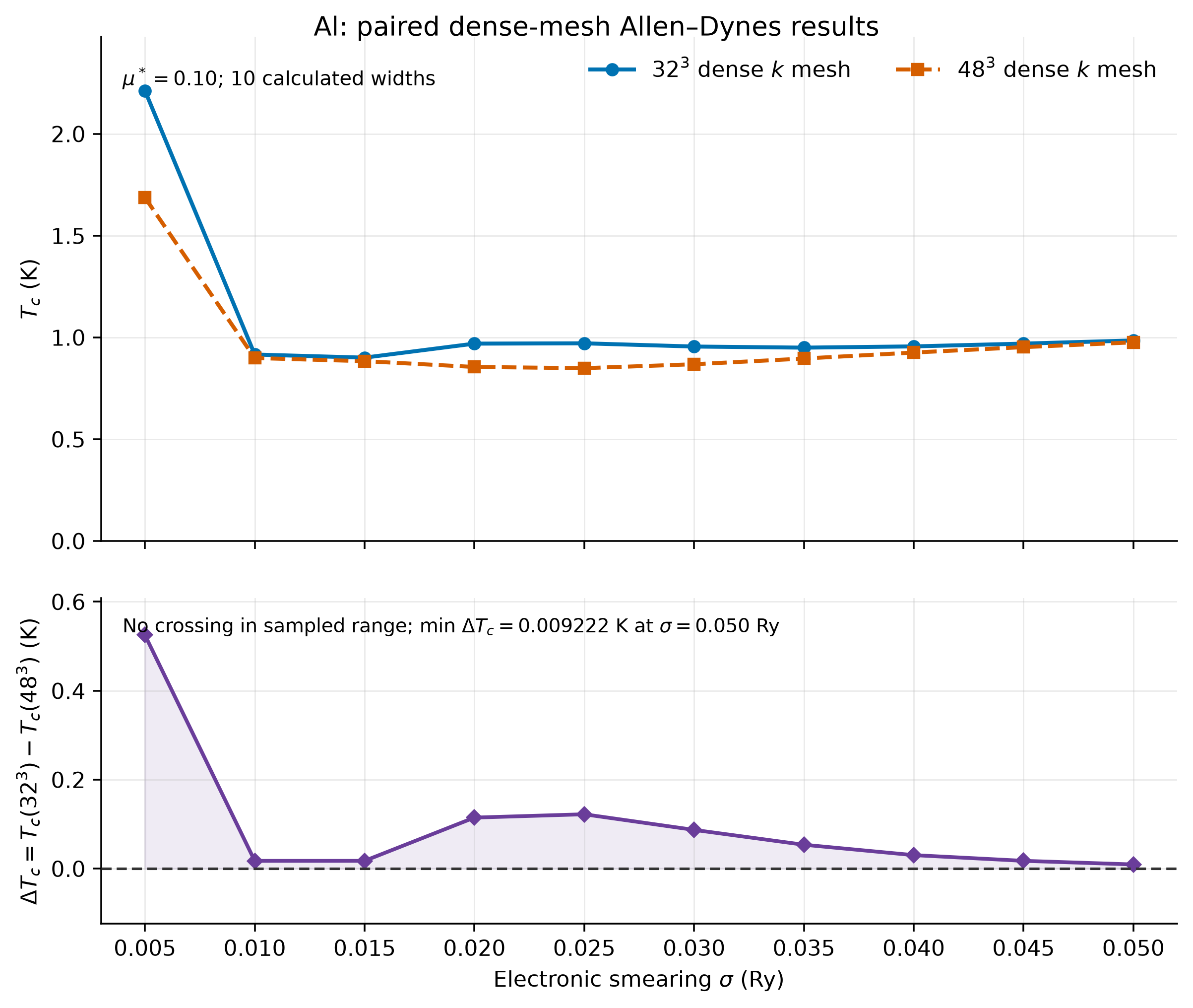
上图每个点都来自对应分支的逐 q EPC 原件。上面把两条 Tc(σ) 放在同一坐标轴,下面画 ΔTc=Tc₃₂−Tc₄₈,虚线为零。十个共同采样点的 ΔTc 均为正;相邻点按直线连接后,0.005–0.050 Ry 内没有交点,也没有重合区间。最接近的位置是 σ=0.050 Ry:Tc₃₂=0.984588 K、Tc₄₈=0.975366 K,ΔTc=+0.009222 K。求交程序同时检查原生三位小数 Tc 与逐 q 重建值,结果一致。
随后计算的 64³ 分支已经完成致密与响应 SCF;ph.x 因三小时 walltime 到限被取消,仅留下六个逐 q EPC 文件,缺少完整八个 q 的结果和 lambda.x 输出。目前图中只有 32³、48³ 两条完整曲线。
配对数值 CSV · 求交结果 JSON · 矢量 PDF · SVG · 完整绘图源码
Tc接近并不一定意味着谱形相同。窄电子展宽把费米面双δ的支撑限制在较少k点上,因而对采样敏感;增大σ能使两条有限网格曲线靠近,也会平滑电子能量选择。要在固定σ下加密k,再检查向较小σ延伸的稳定区;真实q网格与响应k仍各自需要比较。 可以把图中的差异拆回这条公式,看看究竟由哪个输入带来。对相同 μ* 的两条分支,定义 ,便有:
在 σ=0.020 Ry,32³/48³ 的 λqsum 分别是 0.37448594/0.36750469,ωlog 分别为 343.74059/342.62212 K。原件重建表给出的右边两项约为 0.003259 与 0.122563,合计 0.125822,温度比为 1.13408;这对应 0.969044 与 0.854476 K。在这个采样点,主要差别来自指数中的耦合项。其他 σ 应用各自的谱矩重新算,不能沿用本行判断。若两项符号相反,Tc 接近还可能是补偿的结果;下文 σ=0.010 Ry 的谱形比较继续检查这种“一个温度值看不出来”的信息。
按同一 σ 配对,保留全部求交结果
rebuild_tc.py 从八个逐 q 原件重新求和,检查文件头的 q 坐标、权重、展宽、DOS(EF)、模式编号,以及结果是否与原生 λ、ωlog、Tc 的打印精度相符。compare_tc.py 把两边实际写出的 σ 一一配对,保留原生 Tc 与重建值,计算差值并找出所有交点。QE 7.5 lambda.x 源码中的 q 坐标检查被注释掉了;本页的重建脚本逐文件检查坐标和输入顺序,允许六位小数输出带来的舍入差。
两个求和都使用星权重 1, 8, 4, 6, 24, 12, 3, 6,总和 64。程序以总权重归一化,每一档展宽独立求出 λ 和谱函数。计算 Tc 时使用输出括号外的逐 q 加权 λ;括号内的谱积分 λ 用来核对谱积分,不能换掉这一列后继续引用原来的 Tc。
交给代码助手的 Tc 配对、求交与绘图任务
读取 k32/、k48/ 各自的 lambda.in、lambda.out 和八个 elph.inp_lambda 文件,只做保存数据的后处理。核对 q 坐标、顺序、权重、展宽与 μ*,按 QE 7.5 lambda.x 的公式分别重建两条 Tc(σ),并检查原生打印精度。按相同 σ 配对,保存 Tc、λ、ωlog 和逐点 ΔTc。用相邻点的线性差值找出采样范围内所有孤立交点、端点交点和重合区间;若没有交点,明确输出零个,不外推。绘制上方两条 Tc 曲线、下方 ΔTc 与零线,保留十个采样点,用颜色、线型和标记区分分支。保存配对 CSV、求交 JSON、PNG/SVG/PDF 及可独立运行的完整 Python 源码,写明依赖和输入路径;不启动 QE 程序。
已有完整源码:rebuild_tc.py、compare_tc.py、plot_supercon_tc_difference.py。
下载包内已经保留计算结果。在解包目录用完整的 重建脚本 rebuild_tc.py 与配对求交脚本 compare_tc.py 复算表格;这里运行的是读取与求交程序,前面的两次 DFT 计算已在 Maxwell 完成。
$ python3 rebuild_tc.py k32 k48 --outdir comparison-k32-k48
k32:10sigma rows reconstructed; native lambda/omega/Tc match their printed precision
k48:10sigma rows reconstructed; native lambda/omega/Tc match their printed precision
$ python3 compare_tc.py --a k32 --b k48 --out comparison-k32-k48
Paired branches: k32 / k48; 10 common sigma points; mu*=0.10
sigma_Ry  Tc_A_native_K  Tc_B_native_K  Delta_Tc_rebuilt_K
   0.005          2.212          1.687        +0.525165797
   0.010          0.916          0.898        +0.017265344
   0.015          0.900          0.883        +0.017302112
   0.020          0.969          0.854        +0.114568219
   0.025          0.971          0.849        +0.122035939
   0.030          0.955          0.868        +0.086939421
   0.035          0.949          0.896        +0.053537300
   0.040          0.955          0.925        +0.030184671
   0.045          0.969          0.952        +0.017352448
   0.050          0.985          0.975        +0.009221798
All in-range intersections, reconstructed from native elph inputs:
No isolated crossing in the sampled range.
Native 0.001 K print check: 0 isolated points, 0 overlap intervals.
Saved paired-tc.csv, crossings.csv, crossings.json.
从逐点差值求出交点
令 dᵢ = Tc₃₂(σᵢ) − Tc₄₈(σᵢ)。相邻两个采样点的差值异号时,两条折线在这一区间相交:
σ*  = σᵢ − dᵢ × (σᵢ₊₁ − σᵢ) / (dᵢ₊₁ − dᵢ)
Tc* = Tc₃₂(σᵢ) + [Tc₃₂(σᵢ₊₁) − Tc₃₂(σᵢ)] × (σ* − σᵢ) / (σᵢ₊₁ − σᵢ)
这次共同采样范围内没有产生孤立交点,因此没有可代入本式的变号区间。
脚本也保留恰落在采样点上的交点;若相邻采样点连续相等,则记录重合区间。原生打印值、由打印 λ/ωlog 复算的曲线和逐 q 原件重建的曲线分别保存在 JSON 中,方便核对舍入是否改变了交点数或位置。
折线交点表示两条 Tc(σ) 在给定展宽处相等。本页保留这一双网格比较结果;网格收敛还需固定 σ 改变 k/q 网格。EPW 方程页则通过各向同性线性化 Eliashberg 方程本征值穿过 1 来确定临界温度。
再看两条路径的 λ 与 ωlog
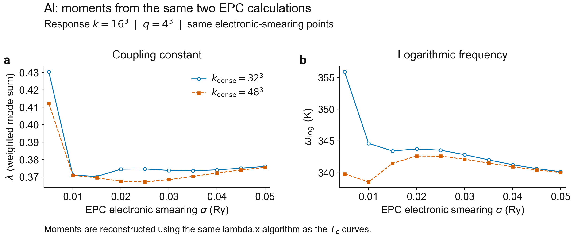
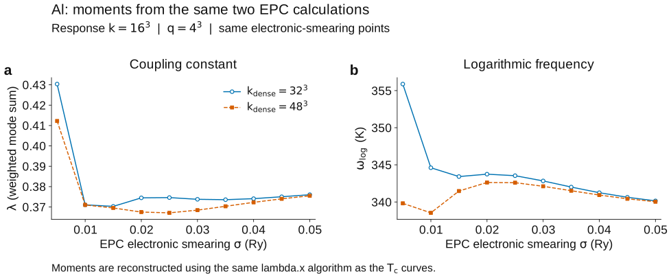
例如,在实际采样的 σ=0.050 Ry 处,32³ 与 48³ 的 λ 分别为 0.376041、0.375505,ωlog 分别为 340.145、340.031 K。本例在十个采样点上,48³ 的 λ 与 ωlog 都低于 32³,二者使 Tc 向同一方向变化。这组数据没有出现两项误差相互抵消形成交点的情况。
本例固定了响应网格和 q 网格;32³ 与 48³ 的致密采样没有交点,不能从中指定一个交点 Tc。QE 官方手册要求检查 k 网格和 Gaussian 展宽,开发者的说明进一步强调固定 σ 的 k 收敛及稳定区向小展宽延伸。若改变真实 q 网格,还要重新核对 k 与展宽。
用谱形、λ 和 ωlog 解释曲线差异
两条 Tc 曲线来自同一公式,差异可以沿 α²F(ω)、耦合积分 λ 和频率矩 ωlog 向上追溯。Poncé 等人的 EPW 论文第 10.3 节、图 12 分别比较 Pb 的采样网格、谱形与 λ,并在充分采样后检查展宽依赖;这里沿用这种分开查看谱与积分的方式,补充解释上面的 Al 双曲线结果。EPW 论文。
本例在相同的十个 σ=0.005–0.050 Ry 上配对 32³ 和 48³ 致密 k 网格的原生 alpha2F.dat。逐频率谱差使用 λ 加权的 L1 距离:
表中百分比为 L1λ 除以两条 λspec 的平均值。ω=0 点两谱均为零,积分从原生 2000 个频率点(0–14 THz)计算,不平滑、不外推。Δ 列统一为 32³−48³。
| σ (Ry) | 谱差 L1 / 平均 λspec (%) | Δλq | Δωlog (K) | ΔTc (K) |
|---|---|---|---|---|
| 0.005 | 35.5188 | +0.018134 | +16.061 | +0.525166 |
| 0.010 | 17.5246 | +0.000072 | +6.072 | +0.017265 |
| 0.015 | 10.4822 | +0.000775 | +1.949 | +0.017302 |
| 0.020 | 5.5562 | +0.006981 | +1.118 | +0.114568 |
| 0.025 | 3.1187 | +0.007491 | +0.939 | +0.122036 |
| 0.030 | 1.9265 | +0.005323 | +0.722 | +0.086939 |
| 0.035 | 1.1384 | +0.003248 | +0.492 | +0.053537 |
| 0.040 | 0.6381 | +0.001806 | +0.312 | +0.030185 |
| 0.045 | 0.3612 | +0.001022 | +0.204 | +0.017352 |
| 0.050 | 0.1903 | +0.000536 | +0.114 | +0.009222 |
σ=0.010 Ry 时,λq 分别为 0.371061(32³)和 0.370989(48³),Δλq 为 +0.000072;谱 L1 为 17.52%,Δωlog 为 +6.072 K。两条谱的权重分布仍有差异,尽管总 λ 很接近。沿这组展宽扫描,谱 L1 从 35.52% 降至 0.19%。这项谱检查解释了相同 σ 下的上游输入差异。
谱数组 alpha2F.dat 以五位小数保存;λq、λspec、ωlog 和 Tc 则由逐 q 的 elph.inp_lambda 原件按 QE 7.5 算法复建。把保存谱直接积分与逐 q 重建的 λspec 对照,最大差为 4.13×10⁻⁶,符合 alpha2F.dat 的打印精度边界。更多有效位用于复算,不代表材料量的物理精度。
十个展宽的完整数值表 · 完整后处理源码 · Tc 配对与交点核验
交给代码助手的谱差补充任务
只做后处理,不启动 pw.x、ph.x、lambda.x 或其他计算程序,也不生成图。读取 k32/alpha2F.dat、k48/alpha2F.dat 和 comparison-k32-k48/paired-tc.csv;验证十档 sigma 一一对应、频率网格相同且覆盖 0–14 THz、所有数值有限。按 L1λ = ∫₀¹⁴ 2|alpha2F32−alpha2F48|/ω dω 计算逐频谱差,并除以两条 lambda_spectrum_rebuilt 的平均值换算百分比;ω=0 且两谱为零时该点被积函数取零。逐档输出 lambda_qsum、lambda_spectrum、omega_log、Tc 的 32³/48³ 数值及差值。检查 alpha2F.dat 直接积分得到的 lambda_spectrum 与 paired-tc.csv 的逐 q 重建值之差,并写明 alpha2F.dat 的五位小数打印精度。保存 spectral-grid-differences.csv 与 spectral-grid-summary.json,保留积分定义、采样点数和频率范围;不做平滑或外推,也不把展宽扫描或无交点写成网格收敛证明。
实际源码 compare_spectral_grids.py 只读上述文件,已生成完整 逐展宽 CSV 与 复算摘要 JSON。运行命令:
python3 compare_spectral_grids.py --root . --outdir comparison-k32-k48
程序逐档打印 λ、谱 L1、Δωlog 和 ΔTc,并保存 CSV/JSON。十档结果及积分误差见上表和摘要文件。
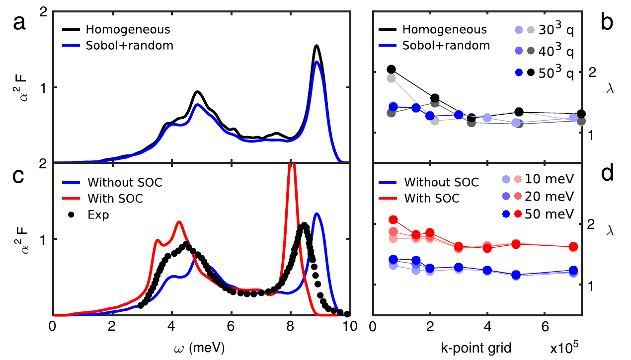
Poncé等,Fig. 12(a,b,d),PDF第12页将三个检查分开:(a)在相同meV频率轴上叠画Pb的α²F,比较均匀与Sobol采样;(b)横轴是电子采样点数,λ按不同q采样分组;(d)在较密采样上改变电子展宽,并分别保留有/无SOC分支。正文第11–12页给出固定0.15 meV声子谱宽,说明不能把电子展宽和谱展宽当同一参数。本页采用(a)先看谱形、再看积分的读法,但横向比较的是Al的32³/48³致密网格,响应16³/q4³固定,原生频率轴为THz。两条链没有Pb的Sobol或SOC比较,图例用本页真实分支身份。
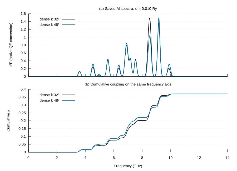
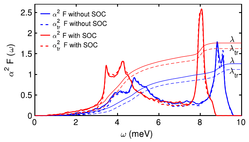
同文Fig. 13,PDF第12页还把普通配对谱与累计λ对读,并在图例中分别标普通配对量和输运谱/输运耦合。本图采用普通α²F与其累计积分,使用两个面板保持各自纵轴,所有数值来自本页Al谱文件。
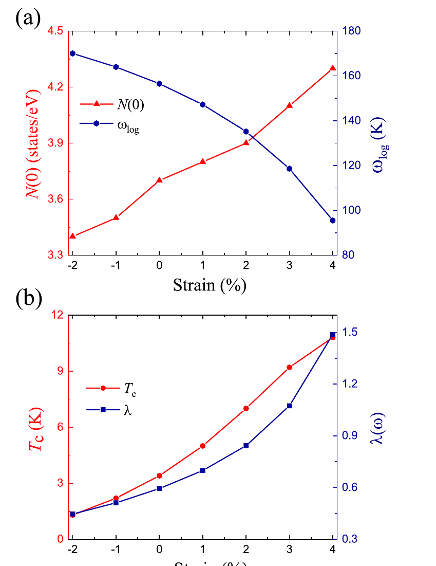
新图可直接看出6–8 THz附近的累计权重差在更高频段得到补偿。按打印谱本身的积分作分母,L1百分比为17.5248%;上表17.5246%沿用原内部重建λspec作分母,差别来自打印精度与离散口径。两者都说明接近的总λ并没有消除频段差异。与Ba₂N Fig. 5(a,b),PDF第4页对读时,注意该图(a)以红/蓝双纵轴分别画N(0)与ωlog,(b)画Tc与λ,横轴是应变;相反的ωlog与λ趋势要通过同一公式解释,而不能按两条线在纸面上的斜率大小比较。本页横轴σ是积分参数,保留上述四个物理量分别核查,不把它称为材料应变趋势。
用保存谱复现这张对照
处理读取双分支包中的 k32/alpha2F.dat 和 k48/alpha2F.dat:首列是 THz 频率,后十列对应电子展宽,第 3 列对应 0.010 Ry。先核对两份表的行列和频率点,再逐点累计 λ,保存原谱与累计值;gnuplot 从这张 CSV 画上下两幅。把两个脚本下载到解包后的 supercon-al-tc 目录,在该目录运行:
python3 prepare_al_spectrum.py --data-dir . --out .
gnuplot plot_al_spectrum.gnuplot
gnuplot -e "export_format='png'" plot_al_spectrum.gnuplot
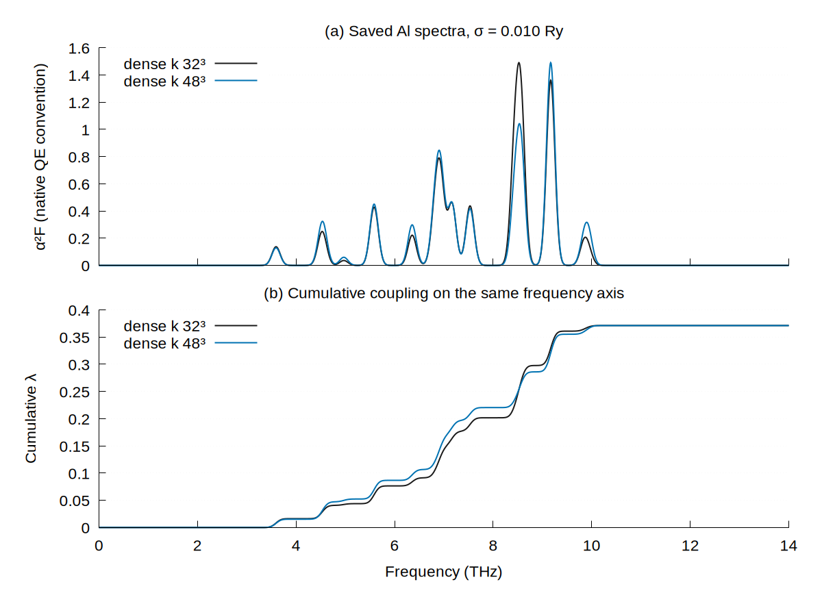
若只看两条累计 λ 的末点,约 17.52% 的谱差如何抵消仍不直观。Poncé等 Fig. 13,PDF第12页在同一 meV 频率轴画普通 α²F 的蓝粗实线与累计 λ 的蓝细实线,输运谱及积分另用虚线,SOC 分支另用红色;这种读法将峰形和已累计的耦合连接起来。本页只分析普通配对谱,保留 Al 原生 THz 横轴,再对两谱取差,将差值累计量放在单独纵轴,便于直接对照增减。
令 ,分别累计其正部 P 与负部的绝对值 N:
于是 ,。P、N 都是谱差的累计量,没有各自归一化成 1;N 以正数表示被减掉的量。
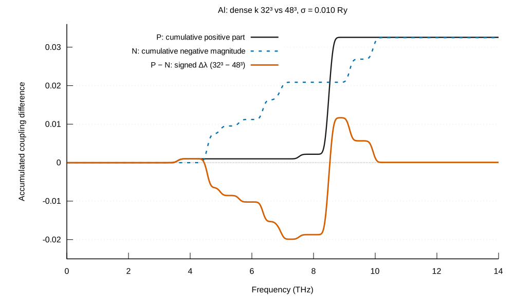
在这张真实数据图中,约 6–8 THz 的净差先偏负,较高频率的正部随后将它抵消。到 14 THz,P=0.03255045、N=0.03248114,而净差仅为 0.00006932;两者相加的 L1=0.06503159 仍较大。这个比较支持“总 λ 接近,却有频段重分布”,不能据它给 Al 指定一个未算出的原子或方向机制。相较于EPW论文 Fig. 12(a),PDF第12页在相同坐标叠画 α²F,本图进一步把本例的差异分解成可复算的积分;这是我们的数据处理,没有假定作者也使用这种分解或公开了作图脚本。
处理程序只读两个原始 2000 行文件,核对同一频率网格和 0.010 Ry 列,在原采样点拆分正负部后作梯形积分;零频点的谱差为零。gnuplot 直接读保存的 CSV,不平滑、不补峰。把完整处理程序与gnuplot 源文件放在双分支包解压目录,运行:
$ python3 spectrum_compensation.py --a k32/alpha2F.dat --b k48/alpha2F.dat --outdir compensation
$ cd compensation
$ gnuplot ../plot_compensation.gnuplot
$ gnuplot -e 'export_format="png"' ../plot_compensation.gnuplot
$ gnuplot -e 'export_format="pdf"' ../plot_compensation.gnuplot
本次使用 gnuplot 6.0。可直接下载逐频率 CSV、积分记录、PNG和183 mm 矢量 PDF。上方原谱图与新积分图来自同一组原件,原谱幅值、累计 λ 和差值各有自己的单位与口径。
σ=0.010 Ry的总λ几乎相同,谱差却为17.52%,ωlog差6.072 K。这说明对总λ的积分会隐藏频段间的补偿;保留谱差和频率矩能解释为何仅检查一个总数不够。0.050 Ry的两条曲线很近,但当前q4³和响应16³固定,无交点与近似重合都没有指定一个收敛材料Tc。
这一步的处理需求可以这样交给编程助手;积分定义和数据列先由我们确定:
读取 k32/alpha2F.dat 与 k48/alpha2F.dat。两份表各有 2000 行频率样本,首列为 THz,表头给出十档电子展宽;提取 0.010 Ry 对应的第 3 列。检查频率严格递增、两表频率逐项一致、谱非负且数值有限。按原频率点用梯形法累计 2α²F(ν)/ν;ν=0 且谱为零时,被积函数取零。输出含频率、两套原谱和两套累计 λ 的 CSV,并另存积分末值和加权谱差。Python 只负责读取、核对和积分,图交给 gnuplot;保留原始采样、幅值与单位。
prepare_al_spectrum.py 完整源码
#!/usr/bin/env python3
"""Prepare a saved Al k32/k48 spectrum comparison; no response calculation.

python3 prepare_al_spectrum.py --data-dir . --out .
Reads the original 2000-row alpha2F.dat of both independent Al chains.
Column 3 (1-based) is sigma=0.010 Ry. No smoothing or spectral normalization.
"""
from pathlib import Path
import argparse, csv, json, math

def load(path):
    lines=path.read_text().splitlines()
    assert lines[0].split()[3]=='0.010', lines[0]
    rows=[[float(x) for x in l.split()] for l in lines[1:] if l.strip()]
    assert len(rows)==2000 and all(len(r)==11 for r in rows)
    assert all(math.isfinite(x) for r in rows for x in r)
    frequency=[r[0] for r in rows]; spectrum=[r[2] for r in rows]
    assert frequency[0]==0 and spectrum[0]==0 and abs(frequency[-1]-14)<1e-8
    assert all(b>a for a,b in zip(frequency,frequency[1:]))
    assert min(spectrum)>=0
    integrand=[0 if f==0 else 2*a/f for f,a in zip(frequency,spectrum)]
    cumulative=[0.0]
    for i in range(1,len(rows)):
        cumulative.append(cumulative[-1]+(frequency[i]-frequency[i-1])*(integrand[i]+integrand[i-1])/2)
    return frequency,spectrum,cumulative

def main():
    parser=argparse.ArgumentParser()
    sources=parser.add_mutually_exclusive_group(required=True)
    sources.add_argument('--data-dir',type=Path,help='Directory containing k32/ and k48/')
    sources.add_argument('--public-root',type=Path,help='Atlas public directory')
    parser.add_argument('--out',type=Path,default=Path('.'))
    args=parser.parse_args();args.out.mkdir(parents=True,exist_ok=True)
    folder=args.data_dir if args.data_dir is not None else args.public_root/'examples/supercon-al-tc'
    x,a,c=load(folder/'k32/alpha2F.dat');y,b,d=load(folder/'k48/alpha2F.dat')
    assert x==y
    with (args.out/'al-sigma010-spectrum.csv').open('w',newline='') as f:
        writer=csv.writer(f)
        writer.writerow(['frequency_THz','alpha2F_k32','alpha2F_k48','lambda_cumulative_k32','lambda_cumulative_k48'])
        writer.writerows(zip(x,a,b,c,d))
    difference=[0 if f==0 else 2*abs(aa-bb)/f for f,aa,bb in zip(x,a,b)]
    l1=sum((x[i]-x[i-1])*(difference[i]+difference[i-1])/2 for i in range(1,len(x)))
    summary={'source_files':['examples/supercon-al-tc/k32/alpha2F.dat','examples/supercon-al-tc/k48/alpha2F.dat'],
             'sigma_Ry':.010,'frequency_unit':'THz','alpha2F':'native lambda.x output convention, no rescaling',
             'lambda_integral':'2 integral alpha2F(f)/f df; trapezoid on original printed frequencies',
             'rows':len(x),'lambda_k32_printed_spectrum':c[-1],'lambda_k48_printed_spectrum':d[-1],
             'L1_lambda':l1,'L1_percent_of_mean_printed_spectrum':l1/((c[-1]+d[-1])/2)*100,
             'normalization':'none; cumulative lambda is dimensionless, separate panel',
             'notes':'This integrates five-decimal printed spectra. Native internal qsum/spec tables retain their own precision.'}
    (args.out/'al-sigma010-summary.json').write_text(json.dumps(summary,indent=2)+'\n')
    print(json.dumps(summary,indent=2))

if __name__=='__main__':main()
plot_al_spectrum.gnuplot 完整源码
# Run beside al-sigma010-spectrum.csv: gnuplot plot_al_spectrum.gnuplot
# Actual run: gnuplot 6.0 patchlevel 0; input is prepared by prepare_al_spectrum.py from saved raw spectra.
set datafile separator comma
set encoding utf8
if (!exists("export_format")) export_format="svg"
if (export_format eq "png") {
    set terminal pngcairo size 1200,866 font "Liberation Sans,17" enhanced
    set output "al-sigma010-spectrum.png"
} else {
    set terminal svg size 900,650 font "Liberation Sans,14" enhanced
    set output "al-sigma010-spectrum.svg"
}
set multiplot layout 2,1 margins 0.12,0.96,0.11,0.92 spacing 0.0,0.075
set xrange [0:14]
set grid ytics lc rgb '#dddddd'
set border 3
set tics nomirror
set key top left opaque
unset xlabel
set format x ''
set ylabel 'α²F (native QE convention)'
set yrange [0:*]
set label 1 '(a) Saved Al spectra, σ = 0.010 Ry' at graph 0.50,1.08 center
plot 'al-sigma010-spectrum.csv' every ::1 using 1:2 with lines lw 2 lc rgb '#1a1a1a' title 'dense k 32³', \
     '' every ::1 using 1:3 with lines lw 2 lc rgb '#0072b2' title 'dense k 48³'
unset label 1
set format x '%g'
set xlabel 'Frequency (THz)'
set ylabel 'Cumulative λ'
set label 1 '(b) Cumulative coupling on the same frequency axis' at graph 0.50,1.08 center
plot 'al-sigma010-spectrum.csv' every ::1 using 1:4 with lines lw 2 lc rgb '#1a1a1a' title 'dense k 32³', \
     '' every ::1 using 1:5 with lines lw 2 lc rgb '#0072b2' title 'dense k 48³'
unset label 1
unset multiplot
unset output
完整源码与重画命令
重建程序保留每个q、模式、星权重和σ;配对程序检查端点、变号区间和连续重合段。相邻点的直线只用来定位当前采样范围内的交点,不外推。绘图读取已有CSV,保留十个样点与ΔTc零线。源码如下,解包后的同一目录也可直接下载并运行。
rebuild_tc.py 的完整源码
#!/usr/bin/env python3
"""Rebuild the QE7.5 lambda.x result from its native elph input files. No QE executable is run."""

import argparse, csv, hashlib, json, math, re
from pathlib import Path

NUMBER = r"[-+]?\d*\.?\d+(?:[EeDd][-+]?\d+)?"
num = lambda x: float(x.replace("D", "E").replace("d", "e"))
sha = lambda p: hashlib.sha256(p.read_bytes()).hexdigest()


def reconstruct(root):
    root = Path(root)
    lines = [
        l.split("!")[0].strip()
        for l in (root / "lambda.in").read_text().splitlines()
        if l.split("!")[0].strip()
    ]
    emax, width, order = map(float, lines[0].split())
    assert order == 0, "This script supports the actual simple-Gaussian spectrum only"
    nq = int(lines[1])
    qs = [list(map(float, l.split())) for l in lines[2 : 2 + nq]]
    names = lines[2 + nq : 2 + 2 * nq]
    mu = float(lines[2 + 2 * nq])
    totalweight = sum(q[3] for q in qs)
    native = (root / "lambda.out").read_text()
    details = re.findall(
        r"lambda\s*=\s*("
        + NUMBER
        + r")\s*\(\s*("
        + NUMBER
        + r")\s*\)\s*<log w>=\s*("
        + NUMBER
        + r")\s*K\s*N\(Ef\)=\s*("
        + NUMBER
        + r")\s*at degauss=\s*("
        + NUMBER
        + r")",
        native,
    )
    printed = [
        list(map(num, line.split()))
        for line in native.split("T_c")[-1].strip().splitlines()
        if len(line.split()) == 3
    ]
    assert len(details) == len(printed) == 10
    n = 2000
    step = emax / (n - 1)
    freq = [i * step for i in range(n)]
    lq = [0.0] * 10
    a2f = [[0.0] * n for _ in range(10)]
    sigma0 = None
    dos0 = None
    ef0 = None
    hashes = {p: sha(root / p) for p in ["lambda.in", "lambda.out"]}
    qcheck = []
    for iq, (qinfo, name) in enumerate(zip(qs, names), 1):
        p = root / name
        hashes[name] = sha(p)
        records = p.read_text().splitlines()
        head = records[0].split()
        qread = list(map(num, head[:3]))
        ns, nm = map(int, head[3:])
        w2 = list(map(num, records[1].split()))
        assert ns == 10 and nm == 3 and len(w2) == 3 and min(w2) >= 0
        coordinate_error = max(abs(x - y) for x, y in zip(qinfo[:3], qread))
        assert (
            coordinate_error <= 5.005e-7
        ), "q differs beyond its six-decimal output rounding"
        weight = qinfo[3] / totalweight
        sig = []
        doses = []
        efs = []
        for j in range(ns):
            k = 2 + j * (nm + 2)
            sm = re.search(
                r"Gaussian Broadening:\s*(" + NUMBER + r") Ry, ngauss=\s*(-?\d+)",
                records[k],
            )
            sigma = num(sm.group(1))
            assert int(sm.group(2)) == 0
            d = re.search(
                r"DOS =\s*(" + NUMBER + r").*at Ef=\s*(" + NUMBER + r")", records[k + 1]
            )
            dos, ef = map(num, d.groups())
            sig.append(sigma)
            doses.append(dos)
            efs.append(ef)
            for im in range(nm):
                m = re.search(
                    r"lambda\(\s*(\d+)\)=\s*("
                    + NUMBER
                    + r")\s*gamma=\s*("
                    + NUMBER
                    + r")",
                    records[k + im + 2],
                )
                assert int(m.group(1)) == im + 1
                lam = num(m.group(2))
                om = math.sqrt(w2[im]) * 3289.828
                lq[j] += weight * lam
                coefficient = weight * lam * om * 0.5 / math.sqrt(math.pi) / width
                for i, e in enumerate(freq):
                    a2f[j][i] += coefficient * math.exp(
                        -min(200.0, ((e - om) / width) ** 2)
                    )
        if sigma0 is None:
            sigma0, dos0, ef0 = sig, doses, efs
        else:
            assert (
                sig == sigma0 and doses == dos0 and efs == ef0
            ), "Sigma/DOS/EF metadata mismatch between q files"
        qcheck.append(
            {
                "q_index": iq,
                "q_lambda_in": qinfo[:3],
                "q_elph": qread,
                "weight": qinfo[3],
                "coordinate_error": coordinate_error,
            }
        )
    rows = []
    for j, detail in enumerate(details):
        lp, l2p, wp, dosp, sigmap = map(num, detail)
        assert sigmap == sigma0[j]
        l2 = 2 * step * sum(a2f[j][i] / freq[i] for i in range(1, n))
        wlog = (
            math.exp(
                2
                * step
                * sum(a2f[j][i] * math.log(freq[i]) / freq[i] for i in range(1, n))
                / l2
            )
            * 47.9924
        )
        value = (
            wlog
            / 1.2
            * math.exp(-1.04 * (1 + lq[j]) / (lq[j] - mu * (1 + 0.62 * lq[j])))
        )
        assert (
            abs(lp - lq[j]) <= 0.500001e-6
            and abs(l2p - l2) <= 0.500001e-6
            and abs(wp - wlog) <= 0.500001e-3
        )
        assert (
            abs(printed[j][2] - value) <= 0.500001e-3
        ), "Reconstruction does not round to native Tc"
        rows.append(
            {
                "sigma_Ry": sigmap,
                "mu_star": mu,
                "lambda_qsum": lq[j],
                "lambda_spectrum": l2,
                "omega_log_K": wlog,
                "N_EF": dosp,
                "N_EF_unit": "states/spin/Ry/cell",
                "Tc_K": value,
                "native_printed_Tc_K": printed[j][2],
                "native_lambda_6dp": lp,
                "native_lambda_spectrum_6dp": l2p,
                "native_omega_log_K_3dp": wp,
                "EF_eV": ef0[j],
            }
        )
    metadata = {
        "source_sha256": hashes,
        "q_pairing": qcheck,
        "q_weight_sum": totalweight,
        "nq": nq,
        "spectrum_points": n,
        "spectrum_max_THz": emax,
        "spectrum_gaussian_width_THz": width,
        "mu_star": mu,
        "formula": "Tc=omega_log/1.2*exp(-1.04*(1+lambda_qsum)/(lambda_qsum-mu_star*(1+0.62*lambda_qsum)))",
        "frequency_constants": "3289.828THz/Ry;47.9924K/THz, matching QE7.5lambda.f90",
        "precision_scope": "Reconstruction of lambda.x from the exact printed elph records, not recovery of unprinted DFT precision. Mode lambda is stored to4decimals; final native Tc is printed to3decimals.",
        "source": "https://github.com/QEF/q-e/blob/qe-7.5/PHonon/PH/lambda.f90",
        "no_QE_executable_run": True,
    }
    return rows, metadata


def main():
    p = argparse.ArgumentParser(description=__doc__)
    p.add_argument(
        "branches",
        nargs="+",
        type=Path,
        help="Directories containing lambda.in/lambda.out/elph_dir",
    )
    p.add_argument("--outdir", type=Path, default=Path("."))
    args = p.parse_args()
    args.outdir.mkdir(parents=True, exist_ok=True)
    for branch in args.branches:
        rows, meta = reconstruct(branch)
        name = branch.name
        with (args.outdir / (name + "-rebuilt.csv")).open("w", newline="") as f:
            w = csv.DictWriter(f, fieldnames=list(rows[0]))
            w.writeheader()
            w.writerows(rows)
        (args.outdir / (name + "-rebuild-checks.json")).write_text(
            json.dumps(meta, indent=2) + "\n"
        )
        print(
            name
            + ":10sigma rows reconstructed; native lambda/omega/Tc match their printed precision"
        )


if __name__ == "__main__":
    main()
compare_tc.py 的完整源码
"""Pair two complete QE lambda.x branches and find straight-segment crossings.

Example, after both independent calculations have completed:
    python3 compare_tc.py --a k32 --b k48 --out comparison

Only Python's standard library is required. Keep rebuild_tc.py beside this
script. Curves reconstructed from lambda.x's actual elph inputs retain the
digits lost by its final 0.001 K printing. Printed Tc and a cross-check from
the printed moments are reported separately, without editing native files.
"""

from pathlib import Path
import argparse
import csv
import hashlib
import json
import math
import re
from rebuild_tc import reconstruct

NUMBER = r"[-+0-9.eEdD]+"
MOMENT = re.compile(
    rf"lambda\s*=\s*({NUMBER})\s*\(\s*({NUMBER})\s*\)\s*"
    rf"<log w>\s*=\s*({NUMBER})\s*K\s*N\(Ef\)\s*=\s*({NUMBER})"
    rf"\s*at degauss=\s*({NUMBER})"
)


def number(value):
    result = float(value.replace("D", "E").replace("d", "e"))
    if not math.isfinite(result):
        raise ValueError("Non-finite native value")
    return result


def digest(path):
    return hashlib.sha256(path.read_bytes()).hexdigest()


def load_branch(path):
    text = (path / "lambda.out").read_text()
    rows = []
    for m in MOMENT.finditer(text):
        lam, spectral_lam, omega, nef, sigma = map(number, m.groups())
        rows.append(
            dict(
                sigma_Ry=sigma,
                lambda_qsum=lam,
                lambda_spectrum=spectral_lam,
                omega_log_K=omega,
                N_Ef_native=nef,
            )
        )
    sections = re.split(r"lambda\s+omega_log\s+T_c", text)
    if len(sections) != 2 or not rows:
        raise ValueError(f"{path}: expected one native Tc table")
    table = []
    for line in sections[1].splitlines():
        if not line.strip():
            continue
        fields = line.split()
        if len(fields) != 3 or not all(re.fullmatch(NUMBER, x) for x in fields):
            raise ValueError(f"{path}: unexpected native Tc row: {line}")
        table.append(list(map(number, fields)))
    if len(table) != len(rows):
        raise ValueError(f"{path}: incomplete moment/Tc pairing")
    sigmas = [r["sigma_Ry"] for r in rows]
    if len(set(sigmas)) != len(sigmas) or sigmas != sorted(sigmas):
        raise ValueError(f"{path}: duplicated or unordered sigma points")
    input_lines = [
        x.split("!")[0].strip() for x in (path / "lambda.in").read_text().splitlines()
    ]
    input_lines = [x for x in input_lines if x]
    mu = number(input_lines[-1])
    for row, (lam, omega, tc) in zip(rows, table):
        # These bounds follow the native five/three-place output formats.
        if abs(row["lambda_qsum"] - lam) > 0.0000051 or row["omega_log_K"] != omega:
            raise ValueError(f"{path}: lambda/Tc table rows do not correspond")
        denominator = row["lambda_qsum"] - mu * (1 + 0.62 * row["lambda_qsum"])
        if denominator <= 0 or omega <= 0 or tc < 0:
            raise ValueError(f"{path}: formula outside the supported positive regime")
        recomputed = (
            omega / 1.2 * math.exp(-1.04 * (1 + row["lambda_qsum"]) / denominator)
        )
        if abs(recomputed - tc) > 0.00055:
            raise ValueError(
                f"{path}: printed moments do not reproduce native Tc rounding"
            )
        row.update(mu_star=mu, Tc_printed_K=tc, Tc_printed_moments_K=recomputed)
    dat = []
    for line in (path / "lambda.dat").read_text().splitlines():
        if line.strip() and not line.lstrip().startswith("#"):
            dat.append(list(map(number, line.split())))
    if len(dat) != len(rows):
        raise ValueError(f"{path}: lambda.dat count mismatch")
    for row, fields in zip(rows, dat):
        expected = [
            row[k]
            for k in (
                "sigma_Ry",
                "lambda_qsum",
                "lambda_spectrum",
                "omega_log_K",
                "N_Ef_native",
            )
        ]
        if fields != expected:
            raise ValueError(f"{path}: lambda.dat differs from stdout")
    return rows, {
        n: digest(path / n) for n in ("lambda.in", "lambda.out", "lambda.dat")
    }


def crossings(x, a, b):
    """Return all isolated sampled zeros, sign changes and overlap intervals."""
    difference = [y - z for y, z in zip(a, b)]
    overlaps = []
    overlap_indices = set()
    for i in range(len(x) - 1):
        if difference[i] == 0 and difference[i + 1] == 0:
            if overlaps and overlaps[-1]["right_index"] == i:
                overlaps[-1].update(sigma_hi_Ry=x[i + 1], right_index=i + 1)
            else:
                overlaps.append(
                    dict(
                        kind="overlap",
                        sigma_lo_Ry=x[i],
                        sigma_hi_Ry=x[i + 1],
                        left_index=i,
                        right_index=i + 1,
                    )
                )
            overlap_indices.update((i, i + 1))
    points = []
    for i, d in enumerate(difference):
        if d == 0 and i not in overlap_indices:
            points.append(
                dict(
                    kind="sampled_equality",
                    sigma_Ry=x[i],
                    Tc_K=a[i],
                    sigma_lo_Ry=x[i],
                    sigma_hi_Ry=x[i],
                    delta_lo_K=0.0,
                    delta_hi_K=0.0,
                )
            )
    for i, (d1, d2) in enumerate(zip(difference, difference[1:])):
        if d1 * d2 < 0:
            t = -d1 / (d2 - d1)
            xc = x[i] + t * (x[i + 1] - x[i])
            ya = a[i] + t * (a[i + 1] - a[i])
            yb = b[i] + t * (b[i + 1] - b[i])
            if not x[i] < xc < x[i + 1] or abs(ya - yb) > 1e-12:
                raise ValueError("Crossing interpolation arithmetic failed")
            points.append(
                dict(
                    kind="segment_crossing",
                    sigma_Ry=xc,
                    Tc_K=ya,
                    sigma_lo_Ry=x[i],
                    sigma_hi_Ry=x[i + 1],
                    delta_lo_K=d1,
                    delta_hi_K=d2,
                )
            )
    points.sort(key=lambda r: r["sigma_Ry"])
    for i, p in enumerate(points, 1):
        p["id"] = f"C{i}"
    return dict(points=points, overlap_intervals=overlaps)


def main():
    parser = argparse.ArgumentParser(description=__doc__)
    parser.add_argument("--a", type=Path, default=Path("k32"))
    parser.add_argument("--b", type=Path, default=Path("k48"))
    parser.add_argument("--out", type=Path, default=Path("comparison"))
    args = parser.parse_args()
    a, ha = load_branch(args.a)
    b, hb = load_branch(args.b)
    xa = [r["sigma_Ry"] for r in a]
    xb = [r["sigma_Ry"] for r in b]
    if xa != xb or {r["mu_star"] for r in a + b} != {a[0]["mu_star"]}:
        raise ValueError("Branches must have identical native sigma values and mu_star")
    # This reconstruction follows the actual QE 7.5 simple-Gaussian inputs.
    # Its own checks compare each result with native output-format precision.
    precise_a, checks_a = reconstruct(args.a)
    precise_b, checks_b = reconstruct(args.b)
    for native, precise in ((a, precise_a), (b, precise_b)):
        if len(native) != len(precise):
            raise ValueError("Incomplete raw-input reconstruction")
        for record, exact in zip(native, precise):
            if (record["sigma_Ry"], record["mu_star"]) != (
                exact["sigma_Ry"],
                exact["mu_star"],
            ):
                raise ValueError(
                    "Raw-input reconstruction is not paired with the native table"
                )
            record.update(
                Tc_rebuilt_K=exact["Tc_K"],
                lambda_qsum_rebuilt=exact["lambda_qsum"],
                lambda_spectrum_rebuilt=exact["lambda_spectrum"],
                omega_log_rebuilt_K=exact["omega_log_K"],
            )
    paired = []
    for ra, rb in zip(a, b):
        row = {"sigma_Ry": ra["sigma_Ry"], "mu_star": ra["mu_star"]}
        for tag, record in [("A", ra), ("B", rb)]:
            row.update({k + "_" + tag: v for k, v in record.items() if k not in row})
        row["delta_Tc_printed_K"] = ra["Tc_printed_K"] - rb["Tc_printed_K"]
        row["delta_Tc_printed_moments_K"] = (
            ra["Tc_printed_moments_K"] - rb["Tc_printed_moments_K"]
        )
        row["delta_Tc_rebuilt_K"] = ra["Tc_rebuilt_K"] - rb["Tc_rebuilt_K"]
        paired.append(row)
    printed = crossings(
        xa, [r["Tc_printed_K"] for r in a], [r["Tc_printed_K"] for r in b]
    )
    reconstructed = crossings(
        xa,
        [r["Tc_printed_moments_K"] for r in a],
        [r["Tc_printed_moments_K"] for r in b],
    )
    raw = crossings(xa, [r["Tc_rebuilt_K"] for r in a], [r["Tc_rebuilt_K"] for r in b])
    report = {
        "branch_A": args.a.name,
        "branch_B": args.b.name,
        "points_per_branch": len(a),
        "mu_star": a[0]["mu_star"],
        "branch_A_hashes": ha,
        "branch_B_hashes": hb,
        "branch_A_rebuild_checks": checks_a,
        "branch_B_rebuild_checks": checks_b,
        "raw_input_reconstruction": raw,
        "native_printed_curves": printed,
        "printed_moment_crosscheck": reconstructed,
        "native_output_files_identical": ha["lambda.out"] == hb["lambda.out"],
        "scope": "All in-range straight-segment intersections; no fit or extrapolation. The plotted curves are reconstructed from exact elph inputs to lambda.x, whose final Tc print precision is 0.001 K. Reconstruction does not recover unprinted DFPT precision. Source files alone do not establish matched protocols: inspect the accompanying independent run review.",
        "scientific_convergence": "not assessed by this postprocessor",
    }
    args.out.mkdir(parents=True, exist_ok=True)
    with (args.out / "paired-tc.csv").open("w", newline="") as f:
        writer = csv.DictWriter(f, fieldnames=list(paired[0]))
        writer.writeheader()
        writer.writerows(paired)
    (args.out / "crossings.json").write_text(json.dumps(report, indent=2) + "\n")
    with (args.out / "crossings.csv").open("w", newline="") as f:
        fields = [
            "id",
            "kind",
            "sigma_Ry",
            "Tc_K",
            "sigma_lo_Ry",
            "sigma_hi_Ry",
            "delta_lo_K",
            "delta_hi_K",
        ]
        writer = csv.DictWriter(f, fieldnames=fields)
        writer.writeheader()
        writer.writerows(raw["points"])
    print(
        f'Paired branches: {args.a.name} / {args.b.name}; {len(a)} common sigma points; mu*={a[0]["mu_star"]:.2f}'
    )
    print("sigma_Ry  Tc_A_native_K  Tc_B_native_K  Delta_Tc_rebuilt_K")
    for row in paired:
        print(
            f'{row["sigma_Ry"]:8.3f}  {row["Tc_printed_K_A"]:13.3f}  {row["Tc_printed_K_B"]:13.3f}  {row["delta_Tc_rebuilt_K"]:+18.9f}'
        )
    print("All in-range intersections, reconstructed from native elph inputs:")
    for p in raw["points"]:
        print(
            f'{p["id"]}: sigma={p["sigma_Ry"]:.9f} Ry; Tc={p["Tc_K"]:.9f} K; bracket=[{p["sigma_lo_Ry"]:.3f}, {p["sigma_hi_Ry"]:.3f}] Ry'
        )
    if not raw["points"]:
        print("No isolated crossing in the sampled range.")
    if raw["overlap_intervals"]:
        print("Overlap intervals:", json.dumps(raw["overlap_intervals"]))
    print(
        f'Native 0.001 K print check: {len(printed["points"])} isolated points, {len(printed["overlap_intervals"])} overlap intervals.'
    )
    print("Saved paired-tc.csv, crossings.csv, crossings.json.")


if __name__ == "__main__":
    main()
compare_spectral_grids.py 的完整源码
#!/usr/bin/env python3
"""Quantify Al k32/k48 Eliashberg spectral and moment differences; no plotting."""
from __future__ import annotations
import argparse, csv, hashlib, json, math
from pathlib import Path

def sha256(path: Path) -> str:
    h = hashlib.sha256()
    with path.open("rb") as f:
        for block in iter(lambda: f.read(1 << 20), b""):
            h.update(block)
    return h.hexdigest()

def read_a2f(path: Path):
    lines = path.read_text().splitlines()
    header = next((line.split() for line in lines if line.strip()), None)
    if not header or len(header) < 3:
        raise ValueError(f"{path}: missing frequency/sigma header")
    sigmas = [float(x) for x in header[2:]]
    groups = {sigma: [] for sigma in sigmas}
    for line in lines[1:]:
        parts = line.split()
        if not parts or parts[0].startswith("#"):
            continue
        values = [float(x) for x in parts]
        if len(values) != len(sigmas) + 1 or any(not math.isfinite(x) for x in values):
            raise ValueError(f"{path}: malformed/non-finite alpha2F row")
        for sigma, a2f in zip(sigmas, values[1:]):
            groups[sigma].append((values[0], a2f))
    for sigma, rows in groups.items():
        xs = [r[0] for r in rows]
        if len(rows) < 2 or any(b <= a for a, b in zip(xs, xs[1:])):
            raise ValueError(f"{path}: invalid frequency axis at sigma={sigma}")
    return groups

def trapezoid(xs, ys):
    return sum((xs[i] - xs[i - 1]) * (ys[i] + ys[i - 1]) / 2 for i in range(1, len(xs)))

def read_pairs(path: Path):
    with path.open(newline="") as f:
        rows = list(csv.DictReader(f))
    return {float(r["sigma_Ry"]): r for r in rows}

def signed_summary(values):
    return {"min": min(values), "max": max(values), "max_abs": max(abs(v) for v in values)}

def main():
    p = argparse.ArgumentParser()
    p.add_argument("--root", type=Path, required=True, help="supercon-al-tc package root")
    p.add_argument("--outdir", type=Path, required=True)
    a = p.parse_args()
    root, outdir = a.root, a.outdir
    outdir.mkdir(parents=True, exist_ok=True)
    path32, path48 = root / "k32/alpha2F.dat", root / "k48/alpha2F.dat"
    s32, s48 = read_a2f(path32), read_a2f(path48)
    paired_path = root / "comparison-k32-k48/paired-tc.csv"
    paired = read_pairs(paired_path)
    sigmas = sorted(set(s32) & set(s48) & set(paired))
    if len(sigmas) != 10 or set(sigmas) != set(s32) or set(sigmas) != set(s48) or set(sigmas) != set(paired):
        raise ValueError("Expected exactly ten common sigma samples in both alpha2F files and paired Tc table")
    result_rows = []
    max_rounded_spectrum_lambda_mismatch = 0.0
    for sigma in sigmas:
        left, right = s32[sigma], s48[sigma]
        if [x[0] for x in left] != [x[0] for x in right]:
            raise ValueError(f"Frequency grids differ at sigma={sigma}")
        row = paired[sigma]
        xs = [r[0] for r in left]
        diff_integrand = [0.0 if x == 0.0 else 2.0 * abs(l[1] - r[1]) / x for x, l, r in zip(xs, left, right)]
        l1 = trapezoid(xs, diff_integrand)
        max_idx = max(range(len(xs)), key=lambda i: abs(left[i][1] - right[i][1]))
        # The native alpha2F.dat prints five decimals; this integral diagnoses spectral-shape
        # differences from that saved output and is not substituted for lambda.x's full-precision moments.
        lam_a2f_32 = trapezoid(xs, [0.0 if x == 0.0 else 2.0 * r[1] / x for x, r in zip(xs, left)])
        lam_a2f_48 = trapezoid(xs, [0.0 if x == 0.0 else 2.0 * r[1] / x for x, r in zip(xs, right)])
        max_rounded_spectrum_lambda_mismatch = max(
            max_rounded_spectrum_lambda_mismatch,
            abs(lam_a2f_32 - float(row["lambda_spectrum_rebuilt_A"])),
            abs(lam_a2f_48 - float(row["lambda_spectrum_rebuilt_B"])),
        )
        record = {
            "sigma_Ry": sigma,
            "lambda_qsum_32": float(row["lambda_qsum_rebuilt_A"]),
            "lambda_qsum_48": float(row["lambda_qsum_rebuilt_B"]),
            "delta_lambda_qsum_32_minus_48": float(row["lambda_qsum_rebuilt_A"]) - float(row["lambda_qsum_rebuilt_B"]),
            "lambda_spectrum_32": float(row["lambda_spectrum_rebuilt_A"]),
            "lambda_spectrum_48": float(row["lambda_spectrum_rebuilt_B"]),
            "delta_lambda_spectrum_32_minus_48": float(row["lambda_spectrum_rebuilt_A"]) - float(row["lambda_spectrum_rebuilt_B"]),
            "weighted_L1_spectral_difference_lambda_from_saved_a2F": l1,
            "weighted_L1_relative_to_mean_lambda_percent": 100.0 * l1 / ((float(row["lambda_spectrum_rebuilt_A"]) + float(row["lambda_spectrum_rebuilt_B"])) / 2.0),
            "max_abs_delta_a2F_from_saved_files": abs(left[max_idx][1] - right[max_idx][1]),
            "frequency_at_max_abs_delta_a2F_THz": xs[max_idx],
            "omega_log_32_K": float(row["omega_log_rebuilt_K_A"]),
            "omega_log_48_K": float(row["omega_log_rebuilt_K_B"]),
            "delta_omega_log_32_minus_48_K": float(row["omega_log_rebuilt_K_A"]) - float(row["omega_log_rebuilt_K_B"]),
            "Tc_32_K": float(row["Tc_rebuilt_K_A"]),
            "Tc_48_K": float(row["Tc_rebuilt_K_B"]),
            "delta_Tc_32_minus_48_K": float(row["Tc_rebuilt_K_A"]) - float(row["Tc_rebuilt_K_B"]),
        }
        result_rows.append(record)
    fields = list(result_rows[0])
    with (outdir / "spectral-grid-differences.csv").open("w", newline="") as f:
        w = csv.DictWriter(f, fieldnames=fields)
        w.writeheader()
        w.writerows(result_rows)
    summary = {
        "method": "For each native sigma, compare the paired saved alpha2F.dat arrays pointwise on their common 0-14 THz grid. Weighted L1 spectral difference is integral 2*abs(alpha2F_32-alpha2F_48)/nu dnu. The source alpha2F.dat values are printed to five decimals; lambda, omega_log and Tc are reconstructed independently from the exact printed elph.inp_lambda records.",
        "source_files": {
            "k32_alpha2F_sha256": sha256(path32),
            "k48_alpha2F_sha256": sha256(path48),
            "paired_tc_sha256": sha256(paired_path),
        },
        "sigma_count": len(result_rows),
        "frequency_bins_per_sigma": len(s32[sigmas[0]]),
        "frequency_range_THz": [s32[sigmas[0]][0][0], s32[sigmas[0]][-1][0]],
        "max_abs_lambda_integral_difference_from_five_decimal_alpha2F_vs_rebuilt_source": max_rounded_spectrum_lambda_mismatch,
        "delta_lambda_qsum_32_minus_48": signed_summary([r["delta_lambda_qsum_32_minus_48"] for r in result_rows]),
        "delta_lambda_spectrum_32_minus_48": signed_summary([r["delta_lambda_spectrum_32_minus_48"] for r in result_rows]),
        "weighted_L1_relative_to_mean_lambda_percent": {
            "min": min(r["weighted_L1_relative_to_mean_lambda_percent"] for r in result_rows),
            "max": max(r["weighted_L1_relative_to_mean_lambda_percent"] for r in result_rows),
            "max_at_sigma_Ry": max(result_rows, key=lambda r: r["weighted_L1_relative_to_mean_lambda_percent"])["sigma_Ry"],
        },
        "delta_omega_log_32_minus_48_K": signed_summary([r["delta_omega_log_32_minus_48_K"] for r in result_rows]),
        "delta_Tc_32_minus_48_K": signed_summary([r["delta_Tc_32_minus_48_K"] for r in result_rows]),
        "tc_curve_crossings": 0 if all(r["delta_Tc_32_minus_48_K"] > 0.0 for r in result_rows) else "review required",
        "interpretation": "This is a dense-k comparison at fixed 16^3 response k, 4^3 q, and common smearing values. It supplies spectral and moment evidence for those two branches, but the smearing scan is not by itself a k/q convergence proof.",
    }
    (outdir / "spectral-grid-summary.json").write_text(json.dumps(summary, indent=2) + "\n")
    print("sigma lambda_q32 lambda_q48 delta_lambda_q L1_spectrum_pct d_omega_log_K delta_Tc_K")
    for r in result_rows:
        print(f"{r['sigma_Ry']:.3f} {r['lambda_qsum_32']:.9f} {r['lambda_qsum_48']:.9f} "
              f"{r['delta_lambda_qsum_32_minus_48']:+.9f} "
              f"{r['weighted_L1_relative_to_mean_lambda_percent']:.5f} "
              f"{r['delta_omega_log_32_minus_48_K']:+.3f} {r['delta_Tc_32_minus_48_K']:+.9f}")
    print(json.dumps(summary, indent=2))

if __name__ == "__main__":
    main()
plot_supercon_tc_difference.py 的完整源码
#!/usr/bin/env python3
"""Plot the paired Al k32/k48 Tc curves and their signed difference."""
from __future__ import annotations
import argparse
import csv
import math
from pathlib import Path

import matplotlib
matplotlib.use("Agg")
import matplotlib.pyplot as plt
from matplotlib.ticker import MultipleLocator


def read_rows(path: Path):
    with path.open(newline="", encoding="utf-8") as f:
        rows = list(csv.DictReader(f))
    if not rows:
        raise ValueError(f"no rows in {path}")
    sigma = [float(r["sigma_Ry"]) for r in rows]
    tc32 = [float(r["Tc_rebuilt_K_A"]) for r in rows]
    tc48 = [float(r["Tc_rebuilt_K_B"]) for r in rows]
    delta_saved = [float(r["delta_Tc_rebuilt_K"]) for r in rows]
    mu = [float(r["mu_star"]) for r in rows]
    if any(not math.isfinite(x) for seq in (sigma, tc32, tc48, delta_saved, mu) for x in seq):
        raise ValueError("non-finite input value")
    if sigma != sorted(sigma) or len(set(sigma)) != len(sigma):
        raise ValueError("sigma values must be strictly increasing")
    if max(mu) - min(mu) > 1e-12:
        raise ValueError("mu* differs between paired rows")
    delta = [a - b for a, b in zip(tc32, tc48)]
    if any(abs(x - y) > 2e-9 for x, y in zip(delta, delta_saved)):
        raise ValueError("stored Delta Tc does not equal Tc32 - Tc48")
    return sigma, tc32, tc48, delta, mu[0]


def intersections(sigma, tc32, tc48):
    if not (len(sigma) == len(tc32) == len(tc48)):
        raise ValueError("paired arrays must have the same length")
    delta = [a - b for a, b in zip(tc32, tc48)]
    points = []
    intervals = []
    i = 0
    while i < len(delta):
        if delta[i] != 0:
            i += 1
            continue
        j = i
        while j + 1 < len(delta) and delta[j + 1] == 0:
            j += 1
        if j > i:
            intervals.append((sigma[i], sigma[j]))
        else:
            points.append((sigma[i], tc32[i]))
        i = j + 1
    for i in range(len(delta) - 1):
        if delta[i] * delta[i + 1] < 0:
            x = sigma[i] - delta[i] * (sigma[i + 1] - sigma[i]) / (delta[i + 1] - delta[i])
            fraction = (x - sigma[i]) / (sigma[i + 1] - sigma[i])
            tc = tc32[i] + fraction * (tc32[i + 1] - tc32[i])
            points.append((x, tc))
    return points, intervals


def main():
    ap = argparse.ArgumentParser()
    ap.add_argument("--data", type=Path, default=Path("comparison-k32-k48/paired-tc.csv"))
    ap.add_argument("--out", type=Path, default=Path("figures"))
    ap.add_argument("--prefix", default="supercon-al-k32-k48-tc-delta")
    args = ap.parse_args()
    sigma, tc32, tc48, delta, mu = read_rows(args.data)
    points, intervals = intersections(sigma, tc32, tc48)
    args.out.mkdir(parents=True, exist_ok=True)

    blue, vermillion = "#0072B2", "#D55E00"
    fig, (ax_tc, ax_delta) = plt.subplots(
        2, 1, figsize=(7.4, 6.1), sharex=True,
        gridspec_kw={"height_ratios": [1.55, 1.0], "hspace": 0.08},
        layout="constrained",
    )
    ax_tc.plot(sigma, tc32, color=blue, marker="o", ms=5, lw=1.8,
               label=r"$32^3$ dense $k$ mesh")
    ax_tc.plot(sigma, tc48, color=vermillion, marker="s", ms=5, lw=1.8,
               ls="--", label=r"$48^3$ dense $k$ mesh")
    ax_tc.set_ylabel(r"$T_c$ (K)")
    ax_tc.set_ylim(0, max(tc32 + tc48) * 1.12)
    ax_tc.legend(frameon=False, ncol=2, loc="upper right")
    ax_tc.text(0.02, 0.94, rf"$\mu^*= {mu:.2f}$; {len(sigma)} calculated widths",
               transform=ax_tc.transAxes, va="top", fontsize=9)

    ax_delta.axhline(0, color="#333333", lw=1.15, ls=(0, (4, 2)), zorder=4)
    ax_delta.plot(sigma, delta, color="#6A3D9A", marker="D", ms=4.5, lw=1.7)
    ax_delta.fill_between(sigma, 0, delta, where=[d >= 0 for d in delta],
                          color="#6A3D9A", alpha=0.10, interpolate=True)
    for x, y in points:
        ax_tc.scatter([x], [y], s=50, facecolor="white", edgecolor="#111111", zorder=5)
        ax_delta.scatter([x], [0.0], s=45, facecolor="white", edgecolor="#111111", zorder=5)
    ax_delta.set_ylabel(r"$\Delta T_c=T_c(32^3)-T_c(48^3)$ (K)")
    ax_delta.set_xlabel(r"Electronic smearing $\sigma$ (Ry)")
    ax_delta.set_xlim(min(sigma) - 0.002, max(sigma) + 0.002)
    ax_delta.xaxis.set_major_locator(MultipleLocator(0.005))
    span = max(delta) - min(delta)
    lo = min(0.0, min(delta)) - 0.24 * span
    hi = max(0.0, max(delta)) + 0.16 * span
    ax_delta.set_ylim(lo, hi)
    if points or intervals:
        summary = f"{len(points)} isolated crossing(s), {len(intervals)} overlap interval(s)"
    else:
        min_i = min(range(len(delta)), key=delta.__getitem__)
        summary = ("No crossing in sampled range; "
                   rf"min $\Delta T_c={delta[min_i]:.6f}$ K at $\sigma={sigma[min_i]:.3f}$ Ry")
    ax_delta.text(0.02, 0.94, summary, transform=ax_delta.transAxes,
                  va="top", fontsize=8.7)
    for ax in (ax_tc, ax_delta):
        ax.grid(axis="both", color="#B7B7B7", alpha=0.28, lw=0.65)
        ax.spines["top"].set_visible(False)
        ax.spines["right"].set_visible(False)
        ax.tick_params(direction="out", length=3.5, width=0.8)
    fig.suptitle("Al: paired dense-mesh Allen–Dynes results", fontsize=12, y=1.015)
    for ext in ("png", "svg", "pdf"):
        fig.savefig(args.out / f"{args.prefix}.{ext}", dpi=320 if ext == "png" else None,
                    bbox_inches="tight")
    plt.close(fig)
    print(f"rows={len(sigma)}; mu*={mu:.2f}; isolated crossings={len(points)}; overlap intervals={len(intervals)}")
    print(f"delta_min_K={min(delta):.9f}; delta_max_K={max(delta):.9f}")
    print(f"saved {args.out / (args.prefix + '.png')}, .svg, .pdf")


if __name__ == "__main__":
    main()
python3 rebuild_tc.py k32 k48 --outdir comparison-k32-k48
python3 compare_tc.py --a k32 --b k48 --out comparison-k32-k48
python3 compare_spectral_grids.py --root . --outdir comparison-k32-k48
python3 plot_supercon_tc_difference.py --data comparison-k32-k48/paired-tc.csv --out figures --prefix supercon-al-k32-k48-tc-delta
前三个处理程序只需Python标准库;绘图需要NumPy、Matplotlib以及包内样式文件。实际终端结果已列在配对段,原始文件和已生成结果在双分支包。含f₁f₂的十档数值与μ*完整表在Al谱矩包的tc-route/data/。
ZrCl₂/Sc₂C保存表怎样使用
前面的三维 Al(32³ 与 48³)在 0.005–0.050 Ry 范围内没有交点。ZrCl₂/Sc₂C 的原始 10 THz ph64/ph96 计算已完成;保存的 18 THz lambdax 表尚未绑定生成输入、运行命令与 QE 可执行文件,ph64.1/ph96.1 曾准备并启动,部分 SCF/PH 输出存在,但没有完整 Tc 输出对。本节报告表格算术与来源边界,不将其称为已验证 Tc。
- 先核对输入参数与保存输出之间的对应关系: ph64/ph96 原始 lambdax.in 首行为 10 0.12 1:emax=10 THz,ngaussq=1 为 Methfessel–Paxton。QE 7.1 lambda.f90 中 ngaussq=0 才是普通 Gaussian。10 THz 输出的谱积分与直接 λ 在全表的差值为 0.015–0.047;18 THz 保存表最大绝对差为 0.000102。高频模式可通过展宽尾部贡献低于 emax 的频率。由于 18 THz 输出没有生成输入、运行命令或 QE 可执行文件记录,不能将两组差异只归因于 emax。参见 QE 7.1 lambda.f90 源码。
- 读取两个 Tc 表的线性插值交点: 按打印到 0.001 K 的 Tc 行分段线性插值,匹配输入的 10 THz 表有两个交点(σ≈0.001750 Ry、Tc≈14.594 K;σ≈0.003091 Ry、Tc≈13.513 K)。来源未闭合的 18 THz 保存表有一个诊断性交点(σ≈0.003579 Ry、Tc≈13.587 K,按两位小数为 13.59 K)。额外插值位数不是物理精度,交点也不能证明 k 网格收敛。Nσ(EF) 在 σ=0.004 与 0.005 Ry 的样点较接近,但不足以宣称进入收敛区。ph64.1/ph96.1 准备输入为 18 0.12 1、el_ph_sigma=0.0005 Ry,目前没有完整 Tc 输出对。
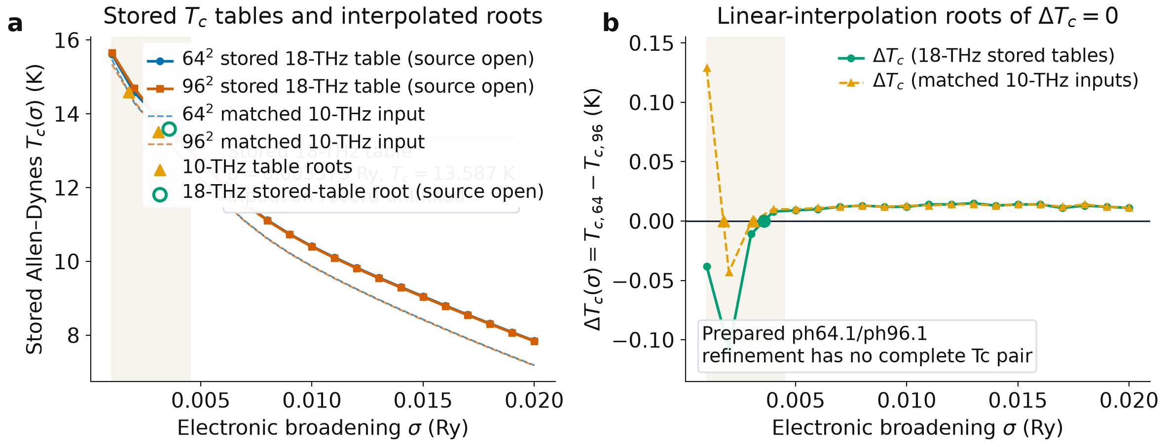
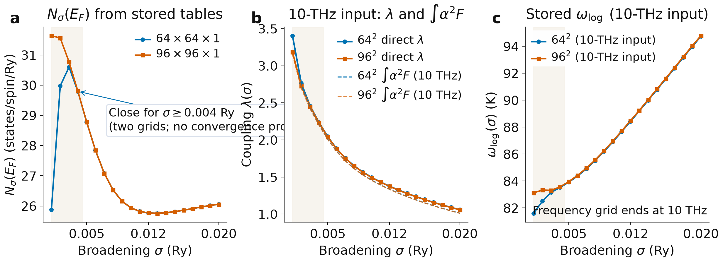
Tc 表算术核对及其来源标记见 tc-intersections.json。可下载 ph64/ph96 保存输出表与绘图脚本;其中 18 THz 输出仍缺生成记录。
这组表保留历史双网格的比较算术,使用它解释交点与谱窗的关系时须同时保留来源标记。ph64/ph96是64²/96²电子网格,q都为8²;它不是q网格收敛对照。新链的中止和现有各向异性EPW准备也不改变这些旧表的接受范围。
公式估计与能隙方程的比较
Ba₂N图3的未应变谱在μ*=0.10简式下给出3.4 K,图7另用各向异性Migdal–Eliashberg方程,能隙在约6 K消失。二者采用不同求解近似;这个文献例子不能给所有材料一个固定修正系数。完整Allen–Dynes用λ、ωlog、二阶矩概括谱,等方方程保留频率核,各向异性方程还保留费米面(n,k)依赖。要只比较求解近似,应保持谱、库仑模型与截断约定一致。
下一页用真实Al谱展示等方EPW的η(T)=1及非线性能隙,并说明怎样走到材料各向异性路线。那里的η=1是方程临界判据;本页两条Tc(σ)求交是电子网格结果相等,二者含义不同。