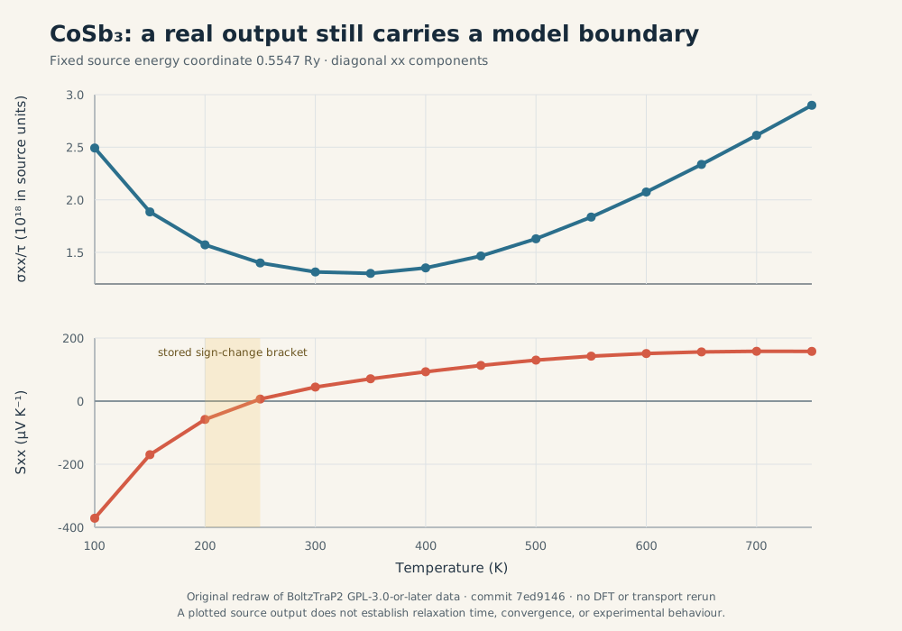
Evidence class: derived-public-data. This example adds a real material transport figure without presenting public output as a calculation performed by this repository. It traces all 14 rows of CoSb3.condtens from the BoltzTraP2 public source archive, stores only the five columns needed here, and generates an original two-panel SVG.
Read the displayed transport object first
Inspect both tensor-component curves with their axes, temperature range, fixed chemical-potential coordinate, and units visible. Ask whether the plotted quantity is absolute or divided by a relaxation time, where the Seebeck sign changes, whether the sampling is dense enough to resolve that feature, and what parent band or scattering information is absent. The figure supports human comparison of two stored trends; it does not show the CoSb3 Fermi surface, k-resolved transport contributions, interpolation error, or a scattering mechanism. See the electronic-transport resources for those routes.
Optional replay after inspecting the published output
python3 examples/practical-guides/boltztrap_cosb3_transport.py \
  --svg public/media/practical-guides/electronic-transport/replot-boltztrap-cosb3-transport/boltztrap-cosb3-transport.svg
The script reads examples/practical-guides/data/boltztrap-cosb3-condtens-20260804.json, checks the frozen source hashes, row and temperature ordering, selected values and sign-change bracket, then writes the SVG. It does not run WIEN2k, BoltzTraP, BoltzTraP2, or a transport convergence study.
Before replaying it, compare the stored JSON header, row count, temperature grid, chemical-potential coordinate, and selected tensor columns with the attributed CoSb3.condtens source. A hash, row, unit, or column mismatch is a provenance failure and should stop the redraw. A mechanism, absolute conductivity, or convergence claim additionally requires the full-zone electronic parent, interpolation record, carrier convention, and compatible scattering or relaxation-time model; this post-processing artifact cannot repair their absence.
Trace the source before interpreting the curves
The BoltzTraP2 public repository is distributed under GPL-3.0-or-later. The frozen source commit is 7ed9146c42d671562daee86d87e253fcbdedaeab. Its data.tar.xz archive had 43,752,436 bytes and SHA-256 ec88d20ae4d00bd58ea98277ef8ee45281eb807160d3955406a819931f3f5169; the extracted member data/CoSb3/CoSb3.condtens had SHA-256 67b6d7e26fa62b4e0a0b56415fa87bade2b764f472b2ed627b09484fa7f81939.
The compact snapshot retains every row and records the source header. The plotted fields are temperature, the diagonal xx conductivity divided by the relaxation time, and the diagonal xx Seebeck coefficient at the output’s fixed chemical-potential coordinate. The original BoltzTraP paper defines the transport approach, while the BoltzTraP2 paper documents the later interpolation and Onsager implementation.
Interpret both panels with their assumptions attached
The source stores sigma_xx/tau, not an absolute conductivity. Its rise or fall cannot be converted to resistivity without a relaxation time that is compatible with the same state, temperature, direction, and scattering model. The Seebeck component is stored in volts per kelvin; the redraw multiplies it by 10^6 and labels microvolts per kelvin.
For this fixed output coordinate, the stored Seebeck values change sign between 200 and 250 K. The script reports that bracket directly from adjacent rows; it does not interpolate a transition temperature or attribute the sign to a unique carrier type. The electron count and thermal occupation change slightly over the series, and the result belongs to the exact source model rather than to all CoSb3 samples.
Inspect the artifact and its assumptions
The standard-library script checks the exact JSON bytes, both recorded source hashes, row count, temperature grid, fixed energy coordinate, selected values, sign-change bracket, and monotonic temperature ordering before redrawing the SVG. The plot footer carries source, licence, commit, and execution boundaries so that a detached image does not become stronger evidence than its data.
What this example does not establish
This repository did not rerun WIEN2k, BoltzTraP, or BoltzTraP2. The example does not establish parent DFT convergence, interpolation accuracy, an absolute relaxation time, scattering-limited conductivity, experimental Seebeck agreement, doping feasibility, thermal stability, or a new conclusion about CoSb3. It is a hash-bound public-output post-processing and provenance test.