For a Fermi-surface claim, inspect a three-dimensional isosurface
Load the dense aluminium mesh into FermiSurfer, XCrySDen, PyProcar, or another suitable viewer, display the Brillouin-zone boundary, and rotate the surface to look for sheets, necks, and pockets. Compare that object with the labelled band path, then change mesh or interpolation settings to see whether features persist. Use electronic-property tools, visual tools, and specialist post-processing tools.
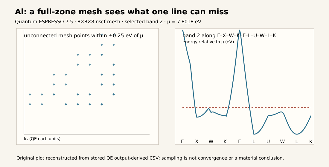
Inspect the stored mesh and path evidence: this page contains a two-dimensional projection of unconnected near-Fermi samples and a separate band path. It contains no three-dimensional isosurface object, exporter output, sheet connectivity, or pocket topology.
Use this real aluminium example when a band-path crossing suggests metallicity or a Fermi-surface feature. It compares separately retained uniform full-zone and path outputs declared for the same model. The public artifacts do not independently prove one continuous historical save-tree ancestry. The point counts and crossings are execution evidence, not a converged isosurface or pocket count.
Purpose
First inspect the committed mesh, path, and receipt without claiming a surface:
head -n 5 examples/practical-guides/data/al-qe/full-zone/al-mesh.csv
head -n 5 examples/practical-guides/data/al-qe/full-zone/al-path.csv
sed -n '1,120p' examples/practical-guides/data/al-qe/full-zone/al-full-zone.json
Judge whether the coordinates, band identity, Fermi marker, point counts, and hashes match the intended state. These tables support sampled crossings only. To make a Fermi-surface claim, export a version-matched regular-grid field to a documented viewer, inspect the three-dimensional object, and test mesh and interpolation sensitivity; until then, stop at the sampled-data description.
For a new calculation, create scf.in from the accepted metallic reference state. Then create nscf.in with a regular full-zone mesh and enough bands for every Fermi-level sheet of interest. The retained Al case used this exact input; all numerical values are case-specific:
&CONTROL
  calculation = 'nscf'
  prefix = 'al'
  pseudo_dir = './pseudo'
  outdir = './tmp'
  verbosity = 'high'
/
&SYSTEM
  ibrav = 2
  celldm(1) = 7.653
  nat = 1
  ntyp = 1
  ecutwfc = 30.0
  ecutrho = 240.0
  occupations = 'smearing'
  smearing = 'mv'
  degauss = 0.02
  nbnd = 4
  nosym = .true.
  noinv = .true.
/
&ELECTRONS
  conv_thr = 1.0d-10
/
ATOMIC_SPECIES
  Al 26.9815385 Al.pbe-n-rrkjus_psl.1.0.0.UPF
ATOMIC_POSITIONS crystal
  Al 0.0 0.0 0.0
K_POINTS automatic
  8 8 8 0 0 0
nosym and noinv retained all 512 points for this direct teaching ledger. They are not a universal requirement: use the downstream exporter’s documented grid requirements, and record whether symmetry reduction is present. The SCF and NSCF must share the compatible cell, pseudopotential, cutoffs, charge, spin/SOC state, occupations, prefix, and accessible outdir.
The recorded QE 7.5 sequence used the explicit fcc primitive-cell state and these program stages in a prepared work directory:
pw.x -in scf.in > scf.out 2> scf.err; printf '%s\n' "$?" > scf.exit
grep -E '^[[:space:]]+convergence has been achieved in[[:space:]]+[0-9]+ iterations[[:space:]]*$' scf.out
grep -F "JOB DONE." scf.out
This creates the parent density. The two grep commands check the reported SCF solver condition and normal termination separately.
pw.x -in nscf.in > nscf.out 2> nscf.err; printf '%s\n' "$?" > nscf.exit
grep -F "JOB DONE." nscf.out
pw.x -in bands.in > bands.out 2> bands.err; printf '%s\n' "$?" > bands.exit
grep -F "JOB DONE." bands.out
The compatible nscf input samples the uniform full-zone state. In this case nosym=.true. and noinv=.true. retain all 512 points for the downstream ledger; that choice is case-specific, not a universal convergence rule. The separate bands input samples 145 points on Gamma-X-W-K-Gamma-L-U-W-L-K. Its crossings describe only those line segments.
The explicit teaching setup uses one Al atom, celldm(1)=7.653 bohr, a PBE ultrasoft pseudopotential, 30 Ry wavefunction cutoff, 240 Ry charge cutoff, Marzari-Vanderbilt smearing of 0.02 Ry, and an 8 x 8 x 8 mesh. These are recorded case values, not transferable recommendations. The pseudopotential filename and SHA-256 are preserved in examples/practical-guides/data/al-qe/full-zone/al-full-zone.json; the potential body is not redistributed.
On HPC, place the same ordered stages in the site’s Slurm template after its module/container setup. Use distinct stdout and stderr, make the job fail after a failed stage, and monitor with the scheduler plus tail -f nscf.out. Before post-processing, inspect all termination and diagonalization signals:
for OUT in scf.out nscf.out bands.out; do
  printf '%s: ' "$OUT"
  grep -F "JOB DONE." "$OUT" | tail -1
done
grep -E '^[[:space:]]+convergence has been achieved in[[:space:]]+[0-9]+ iterations[[:space:]]*$' scf.out | tail -1
grep -Ei "warning|error|stopping|not converged|c_bands" \
  scf.out scf.err nscf.out nscf.err bands.out bands.err || true
grep -F "the Fermi energy is" scf.out nscf.out | tail
The retained Al NSCF and path outputs include c_bands: 1 eigenvalues not converged warnings. JOB DONE. does not clear them. Resolve the electronic diagonalization and rerun before using this case as positive Fermi-surface evidence.
Reconstruct only when source outputs are available
python3 examples/practical-guides/al_qe_full_zone.py \
  --scf-output /path/to/scf.out \
  --mesh-output /path/to/nscf.out \
  --path-output /path/to/bands.out \
  --json examples/practical-guides/data/al-qe/full-zone/al-full-zone.json \
  --mesh-csv examples/practical-guides/data/al-qe/full-zone/al-mesh.csv \
  --path-csv examples/practical-guides/data/al-qe/full-zone/al-path.csv \
  --svg public/media/practical-guides/fermi-surface-and-full-brillouin-zone-analysis/compare-full-zone-isovalue-and-band-path/al-qe-full-zone.svg
The /path/to/... arguments are placeholders for retained source outputs, so this is not the quick inspection command. When those outputs are available, the parser verifies their hashes, the Fermi marker, 512 mesh rows, 145 path rows, and four eigenvalues per row before writing the compact JSON, CSV, and plot. These checks establish dataset identity and shape; they do not establish mesh or isovalue convergence.
The SCF reports a Fermi energy of 7.8018 eV. For selected QE band 2, this run has 237 mesh values below that chemical potential, 275 at or above it, and 48 within the declared +/-0.25 eV teaching window. The ordered path crosses the same value on three sampled intervals. These are observations from this run, not an isosurface, carrier count, or pocket topology.
Keep the scalar field and isovalue together
An equal-energy rendering needs reciprocal coordinates, eigenvalues, band/state identity, and the isovalue from one compatible calculation. Wannier90 documents Fermi-surface output on a regular interpolated grid, and its copper tutorial distinguishes interpolation from direct bands. The present result uses direct pw.x eigenvalues, not Wannier interpolation.
Refine the mesh and perturb the isovalue before naming a pocket, neck, touching, or topology. If interpolation is introduced, compare it with direct eigenvalues near every feature used in the claim. The displayed unconnected scatter preserves the sampled-data boundary; it does not substitute for an isosurface viewer.
Optional documented QE fs.x bridge
The QE PostProc guide documents fs.x as a Fermi-surface exporter that writes a .bxsf file readable by XCrySDen. This public Al case did not run fs.x; it contains no BXSF artifact, so no input or rendered three-dimensional surface is fabricated here. For a new run, use the fs.x input shipped with the exact installed QE release, point it at the completed regular-grid state, and retain its input, stdout, stderr, exit code, and .bxsf file. Then open the BXSF in XCrySDen, display the Brillouin-zone boundary, rotate the object, and inspect sheet connectivity in three dimensions.
Treat exporter completion as file production only. Repeat the SCF/NSCF/export/view sequence for denser regular meshes and for justified changes to the Fermi isovalue or smearing. Record which pockets, necks, or touching features persist; compare exporter/interpolated eigenvalues with direct QE eigenvalues near every claimed feature. If the BXSF is absent, the grid is not compatible, warnings remain, or connectivity changes with resolution, stop the topology or pocket-count claim.
Decide what the example supports
Execution verifies that Quantum ESPRESSO 7.5 completed the recorded SCF, full-zone NSCF, and path programs in the limited sense of normal termination, and that the compact tables reconstruct against the separately recorded source hashes. The unresolved c_bands warnings prevent a clean electronic acceptance. The case supports inspection of a declared sampled mesh/path comparison and its failure signals; it does not establish continuous ancestry, full-zone convergence, a Fermi-surface topology, carrier density, velocity, transport coefficient, interpolation validity, experiment, or an aluminium material conclusion. A high-symmetry path cannot prove full-zone metallicity or the absence of off-path features. The next calculation is a warning-free, denser regular-grid NSCF followed by a real exporter/viewer route and mesh-sensitivity test.