短时 AIMD
Quantum ESPRESSO · Al AIMD 步长对照与界面轨迹判读
方法参考电子自洽 SCF · DFPT 声子与模式分析 · 有限位移声子
层间距会随热运动改变,界面也可能滑移或出现局部重构。研究这些过程时,AIMD 需要同时跟踪原子坐标、温度和电子能量;一条能量曲线有起伏,本身不能说明界面已经保持稳定,也不能说明结构发生了破坏。先确认力与积分能可靠推进轨迹,再读结构随时间的变化。
这里用实际运行的 8 原子周期 fcc Al 学习这一步。它来自 Al 晶胞优化 的单原子原胞,沿三个原胞基矢各重复两次。使用 QE 7.5、LDA-PZ、Al.pz-vbc.UPF、40/160 Ry 截断和 4³ 超胞 k 网格,固定晶胞。已有 100 步 SVR 轨迹和两条相同初态、等时长的 NVE 轨迹;它们检验热浴响应与时间步长误差,时长分别约 97 和 48 fs。
下载完整 Al 计算包,解压后进入 al/aimd。普通电子自洽和弛豫见 SCF 与 固定晶胞优化。研究 ZrCl₂/Sc₂C 或 SnSe₂/Sr₂N 时,初态应来自自身的已接受界面,并重新确定合适的超胞、电子采样、步长和采样窗口;本例的 Al 轨迹不能代表它们的热稳定性。
同一初态使步长比较有意义
8 个原子的初速度来自固定种子 20260922 的正态分布,先减去质心速度,再按 21 个自由度归一化到 300 K。初速度和坐标都写进输入,因此两条 NVE 可以从同一个初态比较步长。最初的输入准备过程保存在 prepare_aimd.py,具体初速度记录在 initial-velocities.json。
下面是最终用于恒温轨迹的完整输入。ATOMIC_POSITIONS crystal 是超胞的分数坐标,ATOMIC_VELOCITIES 使用 QE 的原子单位,不是 Å/fs。
maxwell@maxwell:~/al/aimd/nvt-dt20-cg$ cat al.md.in
&CONTROL
 calculation = 'md'
 nstep = 100
 dt = 20
 iprint = 1
 prefix = 'al'
 pseudo_dir = '<赝势库路径>'
 outdir = './tmp'
 tstress = .true.
 tprnfor = .true.
 verbosity = 'low'
/
&SYSTEM
 ibrav = 0
 nosym = .true.
 nat = 8
 ntyp = 1
 ecutwfc = 40
 ecutrho = 160
 occupations = 'smearing'
 smearing = 'mv'
 degauss = 0.02
 nbnd = 18
/
&ELECTRONS
 diagonalization = 'cg'
 diago_thr_init = 1.0d-9
 diago_full_acc = .true.
 diago_cg_maxiter = 200
 conv_thr = 1.0d-10
/
&IONS
 ion_dynamics = 'verlet'
 ion_velocities = 'from_input'
 ion_temperature = 'svr'
 tempw = 300
 nraise = 20
/
ATOMIC_SPECIES
Al 26.9815385 Al.pz-vbc.UPF
ATOMIC_POSITIONS crystal
Al 0.00000000000000 0.00000000000000 0.00000000000000
Al 0.50000000000000 0.00000000000000 0.00000000000000
Al 0.00000000000000 0.50000000000000 0.00000000000000
Al 0.50000000000000 0.50000000000000 0.00000000000000
Al 0.00000000000000 0.00000000000000 0.50000000000000
Al 0.50000000000000 0.00000000000000 0.50000000000000
Al 0.00000000000000 0.50000000000000 0.50000000000000
Al 0.50000000000000 0.50000000000000 0.50000000000000
CELL_PARAMETERS angstrom
-3.95606780081072 0.00000000000000 3.95606780081072
0.00000000000000 3.95606780081072 3.95606780081072
-3.95606780081072 3.95606780081072 0.00000000000000
K_POINTS automatic
4 4 4 0 0 0
ATOMIC_VELOCITIES
Al -2.96685438852231e-04 5.46443872130152e-04 3.52588534897630e-04
Al 1.83169591108944e-04 -2.23845342698565e-05 3.04783826563648e-04
Al -3.62394243793356e-04 -5.62805162705629e-04 -3.77915518336268e-04
Al 5.62907234083758e-05 9.24073788215892e-05 -1.03170084336693e-04
Al 3.21602394621728e-04 1.76949229988034e-04 3.06925804418459e-05
Al 2.89759188061222e-04 3.51480144555030e-05 -1.67953236314361e-04
Al -1.50927363418241e-04 -2.43518115575532e-04 1.17081675570922e-04
Al -4.08148511364416e-05 -2.22406828442608e-05 -1.56107778486724e-04
calculation='md' 表示晶胞固定的分子动力学。dt=20 使用 pw.x 的 Rydberg 原子时间单位,换算为 0.9675537306 fs;100 步推进的坐标时间为 96.75537306 fs。不能把 20 当成 20 fs,也不能直接套用 cp.x 的 Hartree 原子时间单位。
ion_temperature='svr' 是随机速度缩放温控,tempw=300 设置目标温度,nraise=20 对应约 19.35 fs 的温控特征时间。它不意味着每一步都等于 300 K。这里固定了初速度,没有固定 QE 内部温控的随机数;重新运行这条 SVR 轨迹,逐点温度不会与下面完全重合。
原子运动后不再保持初始空间群
原输入未设置 nosym,原子按不同初速度移动后,第二个几何不满足起始空间群,输出出现:
Error in routine checkallsym (1):
some of the original symmetry operations not satisfied
随后使用 nosym=.true. 的独立目录完成计算。这是运动几何与对称性设置不相容;根据此报错不能判断材料已经发生热破坏。均匀网格的不可约点数随对称性设置改变,电子计算耗时也会变化。数据包保存了初次失败目录与最终输入,重跑时使用下方列出的最终分支。
一次离子推进前,先读电子求解
先取 NVE 大步长分支的第一个离子步。最初的 SCF 已经收敛,紧接着打印能量分解、力与应力。以下是连续输出节选:
!    total energy              =     -33.52087979 Ry
     estimated scf accuracy    <          2.3E-11 Ry
     smearing contrib. (-TS)   =       0.00028280 Ry
     internal energy E=F+TS    =     -33.52116259 Ry

     convergence has been achieved in   8 iterations

     Forces acting on atoms (cartesian axes, Ry/au):

     atom    1 type  1   force =    -0.00000001    0.00000040   -0.00000005
     atom    2 type  1   force =    -0.00000007    0.00000003   -0.00000003
     atom    3 type  1   force =     0.00000000    0.00000004   -0.00000039
     atom    4 type  1   force =    -0.00000038   -0.00000001    0.00000001
     atom    5 type  1   force =     0.00000035   -0.00000005    0.00000002
     atom    6 type  1   force =     0.00000001   -0.00000010    0.00000035
     atom    7 type  1   force =     0.00000006    0.00000003    0.00000001
     atom    8 type  1   force =     0.00000003   -0.00000034    0.00000008

     Total force =     0.000001     Total SCF correction =     0.000004
     SCF correction compared to forces is large: reduce conv_thr to get better values


     Computing stress (Cartesian axis) and pressure

          total   stress  (Ry/bohr**3)                   (kbar)     P=        2.98
   0.00002024   0.00000000   0.00000000            2.98        0.00        0.00
   0.00000000   0.00002024  -0.00000000            0.00        2.98       -0.00
   0.00000000  -0.00000000   0.00002024            0.00       -0.00        2.98


     Molecular Dynamics Calculation
     mass Al               =    26.98
     Time step             =    20.00 a.u.,  0.9676 femto-seconds
estimated scf accuracy 对应电子自洽的残差估计;本例每步要求小于 10⁻¹⁰ Ry。力是接下来推进原子位置所用的量。应力和 P 也会随运动变化,这里固定的是晶胞,不是把压力锁定为零。
这一段还保留了力的警告:初始结构的 Total force 只有约 10⁻⁶ Ry/bohr,而 Total SCF correction 为约 4×10⁻⁶ Ry/bohr,修正相对原力较大。电子残差达到输入阈值,并不能让这条提示自动失效。对本例接近对称极小值的初态,绝对数值很小,但仍不能宣称力已对 conv_thr 收敛;若要研究更精细的动力学量,需要另做更紧电子阈值的力与轨迹对照。后面的减半时间步只检查当前电子设置下的积分误差。
随后出现新的坐标与动能、温度:
Entering Dynamics:    iteration =     1
                           time      =   0.0010 pico-seconds


ATOMIC_POSITIONS (crystal)
Al               0.0001375488        0.0008057202        0.0006561644
Al               0.5001926177        0.0006227609       -0.0006826455
Al               0.0007320655        0.4982569085        0.0002374365
Al               0.4996630927        0.5000608996        0.0001863149
Al              -0.0006258245        0.0007079354        0.4997654513
Al               0.4993407332        0.0002099472        0.4998840831
Al               0.0006842362        0.4996289887        0.4997195349
Al               0.4998755303        0.4997068395        0.5002336603


     kinetic energy (Ekin) =           0.01995091 Ry
     temperature           =         299.99999998 K
     Ekin + Etot (const)   =         -33.50092887 Ry
     Ions kinetic stress =            2.34 (kbar)
                                      2.03           0.64           0.14
                                      0.64           3.10           1.57
                                      0.14           1.57           1.90


     Linear momentum :   -0.0000000000    0.0000000000   -0.0000000000
这里 kinetic energy 是离子动能;电子 SCF 给出的 Etot 与它相加,才是本次 NVE 检查的能量总和。这份八原子、没有固定原子或额外约束、去除质心速度的输入有 个离子自由度,瞬时温度满足 ;用首行的 0.01995091 Ry 可复核约 300 K。QE 7.5 的 compute_ekin 与 get_ndof分别给出温度计算与自由度计数。它是该时刻速度的统计量,和热浴输入的目标温度分开读。金属展宽仍是电子计算中的数值设置,不应把 degauss 换算成离子温度写在这张图上。
前面的 OUT 同时打印了 total energy 与 internal energy E=F+TS。这条有限电子展宽的轨迹使用程序推进离子时对应的 Etot 加离子动能,不把其中一部分时刻换成另一列内部能。此处的 NVE 是固定晶胞、没有离子热浴的积分分支;电子展宽参数仍固定保留,不能进一步称为已经验证的真实有限电子温度系综。
QE 7.5 这段位置 Verlet 输出有一个细节:打印出的新坐标已前进到 n·dt,但同一块里的 Etot 和中心差分速度属于前一个坐标时刻 (n−1)·dt。提取脚本因此分别保存 position_time_fs 与 energy_sample_time_fs;画能量曲线使用后者,导出的坐标轨迹使用前者。这样才能把不同步长的同一物理时刻对齐。
先区分温控交换与积分误差
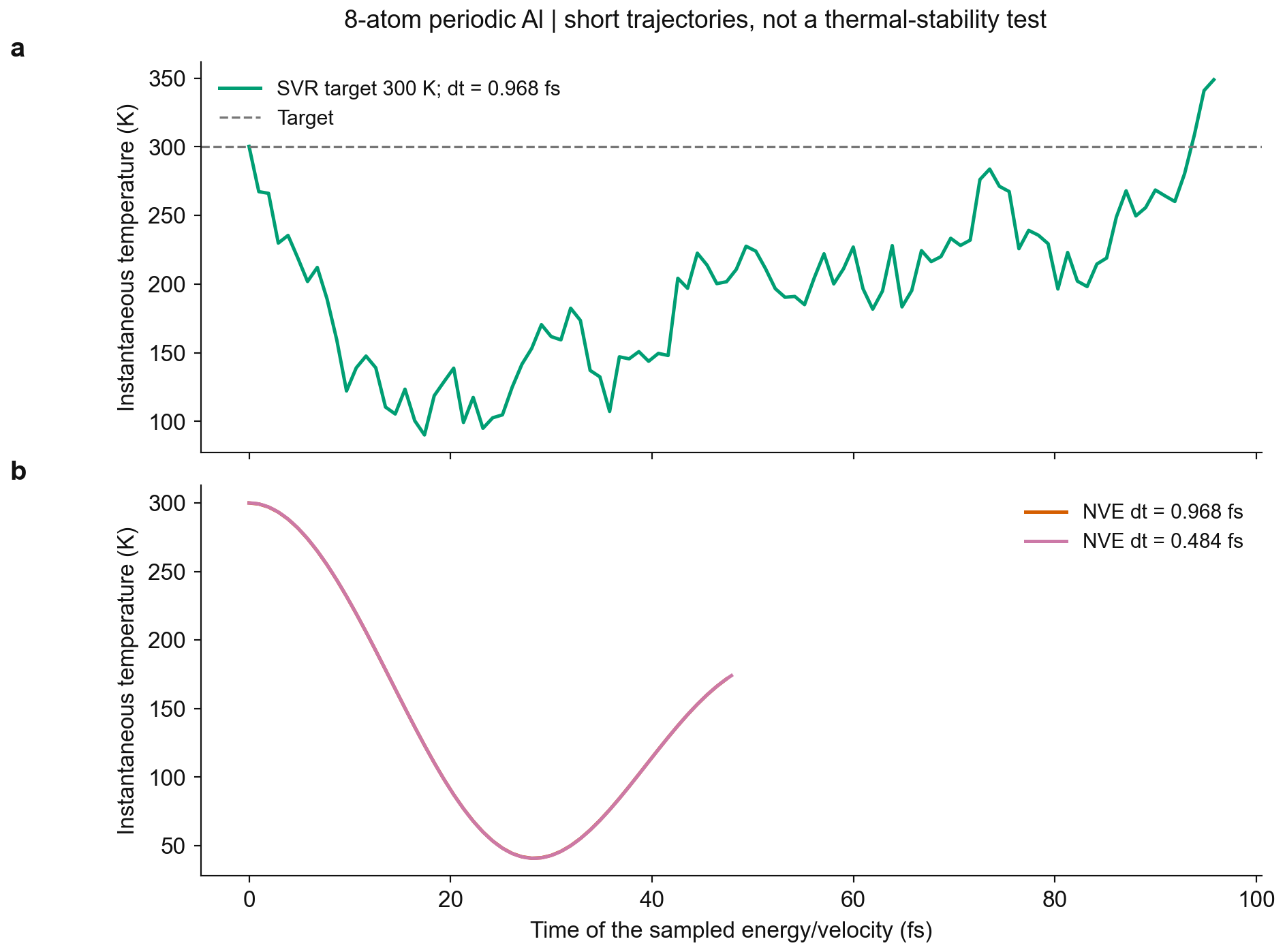
SVR 的输入目标为 300 K,但这段不足 0.1 ps 的实际平均温度只有 196.418 K,瞬时范围为 90.061–348.887 K。它显然还不能作为充分平衡的 300 K 系综。初始位置接近零温极小值,最初输入的动能会转移为位移的势能;8 原子体系也会有很大的瞬时温度起伏。延长平衡与采样、增大体系,并检查统计量才可能回答热平衡性质。
NVE 没有温控,温度从初始 300 K 下降也不自动意味着程序丢失能量。细步长记录在 28.05905819 fs 降到 40.784938 K;相对第一行,离子动能降低 29.317871 meV/atom,电子势能增加 29.321850 meV/atom,总和仅增加 0.003963 meV/atom。势能和动能列分别保留到有限小数位,因此两列差值相加与直接读总能量列之间有末位舍入差别。下面右图把这两列一起画出,方向相反;是否守恒,应看左图里的总和。
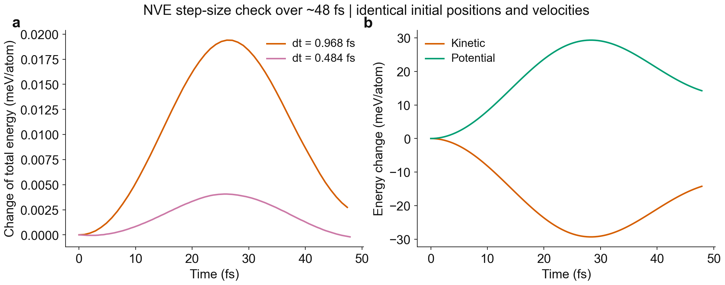
两条 NVE 具有相同初始位置、初速度、电子协议和固定晶胞。大步长设置为 nstep=50, dt=20,小步长设置为 nstep=100, dt=10;两者坐标都推进到 48.377687 fs。
| NVE 步长 | 步数 | 总能量峰峰变化 / meV·atom⁻¹ |
|---|---|---|
| 0.967554 fs | 50 | 0.019405 |
| 0.483777 fs | 100 | 0.004269 |
表中峰峰值取各自完整的能量记录:大步长共 50 个能量时刻,范围为 0–47.410133 fs;小步长共 100 个,范围为 0–47.893910 fs。若只比较共同的 50 个能量时刻 0–47.410133 fs,小步长取 CSV 数据第 1、3、…、99 行,两条记录的峰峰值分别为 0.019405 和 0.004218 meV/atom。这一等时刻对照仍显示减半步长后短程能量波动减小。
坐标检查单独使用两条轨迹的完整末帧:它们都位于 48.377687 fs,原子位置 RMS 差为 2.27×10⁻⁵ Å。这是两个积分步长之间的差;同一条细步长轨迹的末帧相对共同初态,RMS 位移为 0.08657472 Å。原子已经运动,只是两次积分在这个时刻给出了接近的位置。这个共同坐标终点与上面的能量采样终点不同。两项步长对照检验本例短时间内的积分误差;不能把短时波动外推成长期能量稳定,也不能拿 SVR 中随热浴交换而变化的总能量套用 NVE 的守恒要求。
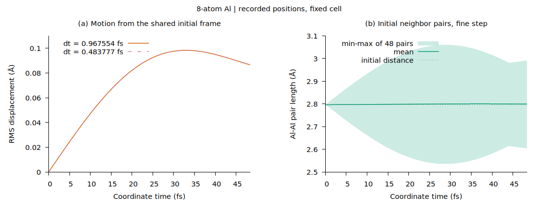
图 (a) 用每一帧相对初态的连续笛卡尔坐标计算 RMS 位移。橙色实线是粗步长,紫色虚线是细步长;两条曲线都在 32.89682684 fs 达到约 0.0983 Å,随后回落,和能量交换一起展示这段实际运动。两条曲线接近到在这个比例下几乎重合,定量差别仍由末帧对照给出。
图 (b) 从初态枚举周期像,选出第一近邻壳层的 48 个不重复 Al–Al 对,沿细步长轨迹追踪相同的原子编号和像平移。初始长度是 2.79736237 Å;末帧平均长度为 2.79985005 Å,但最短、最长分别是 2.60460194 与 2.99119878 Å。绿色均值线变化很小,绿色带却显示各对长度已分散;只报平均值会漏掉这种变化。带的上下边界是这 48 对的最小、最大值,灰色虚线是初始长度,没有统计置信区间的含义。程序始终追踪初始配对,没有重新划分每帧近邻壳层,不能凭这张图宣称配位数不变。
这里两幅横轴都是完整坐标时刻:粗步长有 51 帧,细步长有 101 帧,包含初态和末帧。上面的温度最低点要对应坐标轨迹中同为 28.05905819 fs 的帧,而不是同一打印块里已经推进一次的坐标;末帧则没有对应的最后一条温度、能量记录。
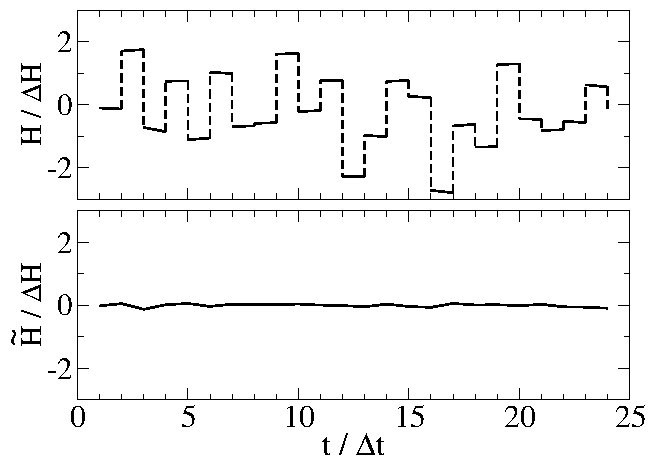
Bussi、Donadio 与 Parrinello,DOI: 10.1063/1.2408420的作者版 PDF 第 4 页 Fig. 1把物理能量 H 与有效守恒量 分成上下两幅:横轴以积分步长计时,纵轴用 H 的均方根涨落归一化;实线段表示 Verlet 推进,虚线段表示速度重标度。这张示意图说明热浴能改变 H,而评估积分误差要跟踪相应守恒量,不能仅凭恒温轨迹的能量线“看着平”作判断。
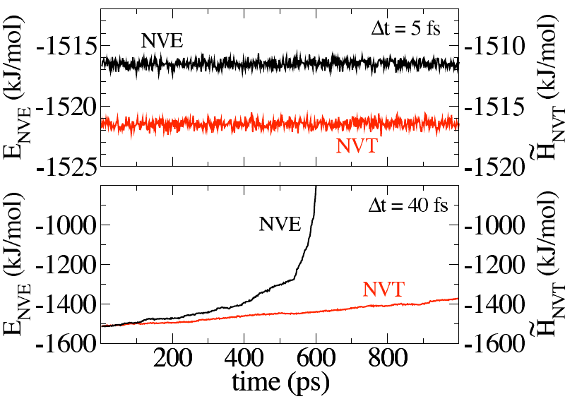
第 5 页 Fig. 2 的上、下两幅使用相同的时间轴(ps),分别展示 5 fs 与 40 fs 的积分步长。每幅黑线对应左轴的 NVE 总能量,红线对应右轴的 SVR–NVT 有效能量,单位均为 kJ/mol;作者比较的是随时间的漂移,而不是把两种纵轴的绝对值相减。小步长没有明显漂移,大步长出现漂移,即使热浴仍让结构轨迹保持有界,也不能据此接受积分精度。本例只对应其中的 NVE 步长检查:已有的两条 Al 轨迹使用相同初态,作图按各自首个能量样本归零、换算为 meV/atom,并对齐真实能量采样时间。没有提取 ,所以不另造 NVT 守恒量曲线,也不用 SVR 的 波动替代它。
提取能量、温度与坐标
每个完成目录都有 al.md.in/out/err。脚本按 MD 步号拆开电子 SCF 与离子输出,读取能量、温度和坐标;保留两个时间字段。坐标属于 ,此处 QE 7.5 的位置 Verlet 输出中能量与中心差分速度属于 。跨步长比较能量时对齐 energy_sample_time_fs,看坐标则使用 position_time_fs。
三条分支共 250 个 SCF 循环均达到了 conv_thr=1e-10 Ry,每步最后一次迭代没有遗留对角化警告。大步长 NVE 的一次中途警告在后续迭代消失;另一个早期 NVT 分支在第 44 步末次迭代仍有警告,保存在包内但没有进入上述结果。程序最后的 JOB DONE. 说明程序正常结束,逐步电子记录才说明这些力由达到当前电子条件的计算给出。
编写 analyse_aimd.py,读取 nvt-dt20-cg、nve-dt20-nosym、nve-dt10-nosym 的最终
al.md.in/out/err;要求分别 100、50、100 个 MD 步、正常步数停止、JOB DONE 和空 stderr。
每步核对电子收敛,区分中途与末次迭代的对角化警告。dt 乘 0.04837768653 得到 fs,
分别保存能量时间 (n-1)*dt 和坐标时间 n*dt;Ry 转 eV,能量差除以 8 个原子。
保存 thermo.csv、连续坐标轨迹和 JSON 摘要;比较 NVE 的等时长能量变化与共同末帧。
保留原始文件,不从不足 0.1 ps 的位移拟合扩散系数或判断长期热稳定性。
analyse_aimd.py 完整源码
from pathlib import Path
import re,csv,json,sys
import numpy as np
r=Path(__file__).resolve().parent
BOHR=0.529177210903;RYEV=13.605693122994;RYTIME_FS=0.04837768653
scenarios=[('nvt-dt20-cg',20.,100),('nve-dt20-nosym',20.,50),('nve-dt10-nosym',10.,100)]
if '--nve-only' in sys.argv: scenarios=scenarios[1:]
all_summary={};all_rows={};all_xyz={}
for name,dt,nstep in scenarios:
    d=r/name;txt=(d/'al.md.out').read_text();inp=(d/'al.md.in').read_text()
    assert 'JOB DONE.' in txt and 'The maximum number of steps has been reached.' in txt
    assert (d/'al.md.err').stat().st_size==0
    assert not re.search(r'convergence NOT achieved|Error in routine',txt)
    starts=list(re.finditer(r'Entering Dynamics:\s+iteration\s*=\s*(\d+)',txt));assert len(starts)==nstep
    cellblock=inp.split('CELL_PARAMETERS angstrom')[1].split('K_POINTS')[0]
    cell=np.array([list(map(float,l.split())) for l in cellblock.strip().splitlines()])
    init=np.array([list(map(float,l.split()[1:4])) for l in inp.split('ATOMIC_POSITIONS crystal')[1].split('CELL_PARAMETERS')[0].strip().splitlines()])
    assert init.shape==(8,3) and cell.shape==(3,3)
    nconv=len(re.findall(r'convergence has been achieved in\s+(\d+) iterations',txt));assert nconv==nstep
    rows=[];positions=[init@cell]
    for i,m in enumerate(starts):
        step=int(m.group(1));assert step==i+1
        pre=txt[(starts[i-1].end() if i else 0):m.start()]
        end=starts[i+1].start() if i+1<len(starts) else len(txt)
        b=txt[m.start():end]
        potential=float(re.findall(r'!\s+total energy\s*=\s*([-\d.]+)\s+Ry',pre)[-1])
        kinetic=float(re.search(r'kinetic energy \(Ekin\)\s*=\s*([-\d.]+)',b).group(1))
        total=float(re.search(r'Ekin \+ Etot \(const\)\s*=\s*([-\d.]+)',b).group(1))
        temperature=float(re.search(r'temperature\s*=\s*([-\d.]+)\s*K',b).group(1))
        assert abs(total-(potential+kinetic))<2e-8
        assert 'eigenvalues not converged' not in re.split(r'iteration\s+#\s*\d+',pre)[-1]
        early_warnings=pre.count('eigenvalues not converged')
        conv=int(re.findall(r'convergence has been achieved in\s+(\d+) iterations',pre)[-1])
        residual=float(re.findall(r'estimated scf accuracy\s*<\s*([.\dEe+\-]+)\s*Ry',pre)[-1])
        assert residual<=1.0e-10
        posblock=b.split('ATOMIC_POSITIONS (crystal)')[1].strip().splitlines()[:8]
        frac=np.array([list(map(float,l.split()[1:4])) for l in posblock]);assert frac.shape==(8,3)
        positions.append(frac@cell)
        # Position-Verlet in QE 7.5 advances coordinates before output_tau.
        # Etot and the centred finite-difference velocity belong to the preceding position.
        rows.append(dict(step=step,energy_sample_time_fs=(step-1)*dt*RYTIME_FS,position_time_fs=step*dt*RYTIME_FS,temperature_K=temperature,potential_Ry=potential,kinetic_Ry=kinetic,total_Ry=total,scf_iterations=conv,early_diagonalization_warning_count=early_warnings,scf_estimated_accuracy_Ry=residual))
    t=np.array([v['energy_sample_time_fs'] for v in rows]);en=np.array([v['total_Ry'] for v in rows]);temps=np.array([v['temperature_K'] for v in rows]);de=(en-en[0])*RYEV*1000/8
    for v,x in zip(rows,de):v['total_change_meV_atom']=float(x)
    with (d/'thermo.csv').open('w') as f:
        w=csv.DictWriter(f,fieldnames=rows[0].keys());w.writeheader();w.writerows(rows)
    xyz=np.array(positions);np.savez_compressed(d/'trajectory.npz',positions_A=xyz,cell_A=cell,time_fs=np.arange(nstep+1)*dt*RYTIME_FS)
    lattice=' '.join(f'{v:.12f}' for v in cell.ravel())
    with (d/'trajectory.xyz').open('w') as f:
        for j,pos in enumerate(xyz):
            f.write('8\nLattice="'+lattice+'" Properties=species:S:1:pos:R:3 pbc="T T T" time_fs='+str(j*dt*RYTIME_FS)+'\n')
            f.writelines('Al '+' '.join(f'{x:.10f}' for x in p)+'\n' for p in pos)
    wall=re.findall(r'PWSCF\s*:\s*(.*?)\s+CPU\s+(.*?)\s+WALL',txt)[-1][1]
    summary=dict(nsteps=nstep,natoms=8,dt_Ry_au=dt,dt_fs=dt*RYTIME_FS,coordinate_end_time_fs=nstep*dt*RYTIME_FS,energy_end_time_fs=float(t[-1]),all_scf_converged=True,final_scf_iteration_diagonalization_warnings=0,early_scf_diagonalization_warnings=sum(v['early_diagonalization_warning_count'] for v in rows),scf_cycles=nconv,scf_iterations_min=min(x['scf_iterations'] for x in rows),scf_iterations_max=max(x['scf_iterations'] for x in rows),temperature_first_K=float(temps[0]),temperature_mean_K=float(np.mean(temps)),temperature_min_K=float(np.min(temps)),temperature_max_K=float(np.max(temps)),temperature_last_K=float(temps[-1]),energy_change_final_meV_atom=float(de[-1]),energy_peak_to_peak_meV_atom=float(np.ptp(de)),energy_linear_slope_meV_atom_ps=float(np.polyfit(t,de,1)[0]*1000),rms_displacement_final_A=float(np.sqrt(np.mean(np.sum((xyz[-1]-xyz[0])**2,axis=1)))),max_atom_displacement_A=float(np.max(np.linalg.norm(xyz[-1]-xyz[0],axis=1))),wall_time=wall,interpretation='short fixed-volume small-cell trajectory; not thermal-stability or equilibrium-property evidence')
    (d/'summary.json').write_text(json.dumps(summary,indent=2)+'\n');all_summary[name]=summary;all_rows[name]=rows;all_xyz[name]=xyz
coarse=np.array([v['total_change_meV_atom'] for v in all_rows['nve-dt20-nosym']]);fine=np.array([v['total_change_meV_atom'] for v in all_rows['nve-dt10-nosym'][::2]])
assert coarse.shape==fine.shape
matched=dict(matched_energy_times=50,energy_time_end_fs=all_rows['nve-dt20-nosym'][-1]['energy_sample_time_fs'],max_energy_change_difference_meV_atom=float(np.max(np.abs(coarse-fine))),final_position_same_time_fs=all_summary['nve-dt20-nosym']['coordinate_end_time_fs'],rms_position_difference_at_same_end_A=float(np.sqrt(np.mean(np.sum((all_xyz['nve-dt20-nosym'][-1]-all_xyz['nve-dt10-nosym'][-1])**2,axis=1)))))
all_summary['nve_matched_time_comparison']=matched
all_summary['time_axis_note']='QE7.5 position Verlet prints advanced coordinates at n*dt; Etot and centred velocity in that block refer to preceding geometry at (n-1)*dt. CSV keeps both clocks.'
(r/'summary.json').write_text(json.dumps(all_summary,indent=2)+'\n')
print('case                steps  dt_fs    coord_end_fs  energy_range_meV_atom  mean_T_K')
for name,s in all_summary.items():
    if not isinstance(s,dict) or 'nsteps' not in s:continue
    print(f"{name:20s} {s['nsteps']:3d}  {s['dt_fs']:.6f}  {s['coordinate_end_time_fs']:9.6f}  {s['energy_peak_to_peak_meV_atom']:13.6f}       {s['temperature_mean_K']:.3f}")
print(f"All {sum(n for _,_,n in scenarios)} SCF cycles converged; no final-iteration diagonalization warning; {len(scenarios)} native JOB DONE endings.")
print('Early SCF diagonalization warnings:', {n: all_summary[n]['early_scf_diagonalization_warnings'] for n,_,_ in scenarios})
print('NVE position difference at the common final time:',matched['rms_position_difference_at_same_end_A'],'angstrom RMS')
print('NVE total-energy conservation tested only over ~48 fs; no thermodynamic convergence claim.')
提取程序使用 Python 3 与 NumPy。原图生成记录使用 Matplotlib;下面的 gnuplot 重画路线直接读取提取好的 CSV。保留数据包的目录层级,在 al/aimd 目录运行:
python3 analyse_aimd.py
实际输出为:
case                steps  dt_fs    coord_end_fs  energy_range_meV_atom  mean_T_K
nvt-dt20-cg          100  0.967554  96.755373      51.897811       196.418
nve-dt20-nosym        50  0.967554  48.377687       0.019405       142.856
nve-dt10-nosym       100  0.483777  48.377687       0.004269       142.226
All 250 SCF cycles converged; no final-iteration diagonalization warning; 3 native JOB DONE endings.
NVT 的 51.897811 meV/atom 范围包含热浴交换,不能与 NVE 的守恒误差放在同一标准下排名。结果还保存在各分支的 thermo.csv 与 summary.json。坐标 XYZ 含初始帧及所有推进帧,三条分支分别有 101、51、101 帧;连续未回卷坐标被保留,避免周期边界跳转被当成突然运动。
| 分支 | 输入与脚本 | 完整 OUT | 数值与坐标 |
|---|---|---|---|
| nvt-dt20-cg | 输入 / 脚本 | OUT | CSV / XYZ |
| nve-dt20-nosym | 输入 / 脚本 | OUT | CSV / XYZ |
| nve-dt10-nosym | 输入 / 脚本 | OUT | CSV / XYZ |
完整 MPI 和环境设置见每条分支自己的 run.slurm。恒温分支原记录使用 16 个 MPI 进程、8 个 k 点池,两个 NVE 使用 8 个 MPI 进程;所有分支每进程一个 OpenMP 线程。重新计算前应修改实际程序与赝势路径。已有数据的提取和重画不需要提交这些作业。
用实际数据重画积分对照
温度图使用 CSV 的真实采样时间;NVE 总能量以各自第一行作差,再转成 meV/atom。势能和动能交换图也取同一基准。Bussi Fig. 2 的比较方法在这里落实为共同时间轴和独立的能量零点,单位使用本例的每原子能量,不借用论文模型的 kJ/mol 数值。
把 gnuplot 完整脚本保存到 al 根目录,目录中应保留 aimd/nve-dt20-nosym/thermo.csv 和 aimd/nve-dt10-nosym/thermo.csv。运行:
gnuplot plot_aimd.gp
输出的 al-nve-gnuplot.svg/png/pdf 分两幅:左幅用 CSV 的第 2 列 energy_sample_time_fs 和第 11 列 total_change_meV_atom;细步长每隔一个样本取一点,与粗步长对齐到 50 个共同时间,终点 47.4101327994 fs。右幅用细步长的势能、动能列分别减去首行,再乘 Ry→eV→meV/atom 的系数,显示两者怎样交换。左幅相同窗口内的峰峰变化分别为 0.019405 与 0.004218 meV/atom;正文原图和上表的细步长 0.004269 使用全部 100 行,末个能量时刻为 47.8939096647 fs。两个窗口保留各自定义,不通过插值制造共同点。坐标的短时 RMS 位移仍只用于轨迹核对,不能将其斜率直接换成扩散系数。
plot_aimd.gp 完整源码
# Use energy_sample_time_fs, not position_time_fs.
if (!exists("data_root")) data_root = "."
if (!exists("out_root")) out_root = "."
coarse = data_root."/aimd/nve-dt20-nosym/thermo.csv"
fine = data_root."/aimd/nve-dt10-nosym/thermo.csv"
set encoding utf8
set datafile separator ","
set datafile columnheaders
stats fine using ($1==1 ? $5 : 1/0) nooutput
p0 = STATS_mean
stats fine using ($1==1 ? $6 : 1/0) nooutput
k0 = STATS_mean
conv = 13.605693122994*1000/8
set border 3
set tics out nomirror
set key top left
do for [ext in "svg png pdf"] {
    if (ext eq "svg") { set terminal svg size 1000,400 enhanced font "DejaVu Sans,11" }
    if (ext eq "png") { set terminal pngcairo size 1000,400 enhanced font "DejaVu Sans,11" }
    if (ext eq "pdf") { set terminal pdfcairo size 10,4 enhanced font "DejaVu Sans,11" }
    set output out_root."/al-nve-gnuplot.".ext
    set size 1,1
    set origin 0,0
    unset title
    set multiplot layout 1,2 margins 0.11,0.98,0.18,0.82 spacing 0.14,0.05 title "8-atom Al | existing short NVE records"
    set title "(a) 50 matched energy times"
    set xlabel "Energy sample time (fs)"
    set ylabel "Change of total energy (meV/atom)"
    set xrange [0:47.4101328]
    set yrange [-0.002:0.022]
    plot coarse using 2:11 with linespoints pt 7 ps 0.3 lw 1 lc rgb "#D55E00" title "dt = 0.967554 fs", fine every 2 using 2:11 with linespoints pt 5 ps 0.3 lw 1 lc rgb "#CC79A7" title "dt = 0.483777 fs"
    set title "(b) Energy exchange, fine step"
    set ylabel "Change from first sample (meV/atom)"
    set xrange [0:47.8939097]
    set yrange [*:*]
    plot fine using 2:(($5-p0)*conv) with lines lw 1 lc rgb "#009E73" title "Potential", fine using 2:(($6-k0)*conv) with lines lw 1 lc rgb "#D55E00" title "Kinetic"
    unset multiplot
    unset output
}
print "Wrote al-nve-gnuplot.svg/.png/.pdf; panel (a) uses 50 shared energy times"
上述结构图可从已有 NPZ 与 CSV 独立复现。把 结构提取脚本与 gnuplot 脚本保存到 al 根目录;前者需要 Python 3 和 NumPy,后者需要 gnuplot。它们读取两条 NVE 分支,不推进原子:
python3 inspect_aimd_observables.py
gnuplot plot_aimd_structure.gp
实际提取输出为:
nve-dt20-nosym: frames=51 initial_pairs=48 initial_nn=2.79736237 A
  RMS_end=0.08658109 A RMS_peak=0.09833092 A at 32.89682684 fs
  end_initial_neighbor_range=2.60455756..2.99124352 A
nve-dt10-nosym: frames=101 initial_pairs=48 initial_nn=2.79736237 A
  RMS_end=0.08657472 A RMS_peak=0.09831608 A at 32.89682684 fs
  end_initial_neighbor_range=2.60460194..2.99119878 A
matched_end_RMS_difference=2.2722030842e-05 A
输出在 structure-observations:两份结构 CSV、JSON 摘要与 SVG/PNG/PDF 图。细步长 CSV与 JSON 摘要保留图中数值、温度最低点及其同时间结构帧。CSV 最后一帧的温度栏留空,因为原输出没有与它同时间的温度样本。
给编程助手的要求可以具体到配对与时间的处理:
读取已有 Al 两条 NVE 的 trajectory.npz 和 thermo.csv,核对晶胞、帧数与独立时间轴。保留未回卷坐标,算每帧相对初态的 RMS 位移。对初态枚举每个方向 −1、0、1 的周期像,选择最短壳层,去掉互为反向的重复对;追踪这 48 对的固定编号和像平移,输出最短、最长和均值。温度用同坐标时刻的能量行匹配,最后坐标帧没有样本就留空。记录最低温度时的动势能差与位置,两种步长的末帧另作对照。用 gnuplot 画位移曲线和近邻对长度范围,不把固定配对称为逐帧配位判据,不从短时位移拟合扩散。
inspect_aimd_observables.py 完整源码
"""Inspect existing Al trajectory frames and match their native energy clock."""
from pathlib import Path
import csv, itertools, json, sys
import numpy as np

root = Path(sys.argv[1]) if len(sys.argv) > 1 else Path(".")
out = Path(sys.argv[2]) if len(sys.argv) > 2 else Path("structure-observations")
out.mkdir(parents=True, exist_ok=True)
cases = ("nve-dt20-nosym", "nve-dt10-nosym")
summary = {}
end_frames = {}
for case in cases:
    folder = root / "aimd" / case
    thermo = list(csv.DictReader((folder / "thermo.csv").open()))
    with np.load(folder / "trajectory.npz") as trajectory:
        positions = trajectory["positions_A"]
        cell = trajectory["cell_A"]
        time = trajectory["time_fs"]
    assert positions.shape == (len(thermo) + 1, 8, 3)
    assert cell.shape == (3, 3) and np.isfinite(positions).all()
    assert all(abs(float(row["energy_sample_time_fs"]) - time[j]) < 1e-8 for j, row in enumerate(thermo))
    # Use explicit periodic images; component-wise rounding is unsuitable for this oblique cell.
    candidates = []
    for i, j, shift in itertools.product(range(8), range(8), itertools.product((-1, 0, 1), repeat=3)):
        if i == j and shift == (0, 0, 0):
            continue
        vector = positions[0, j] - positions[0, i] + np.array(shift) @ cell
        candidates.append((float(np.linalg.norm(vector)), i, j, shift))
    nearest = min(item[0] for item in candidates)
    bonds = []
    for distance, i, j, shift in candidates:
        reverse = (j, i, tuple(-n for n in shift))
        if abs(distance - nearest) < 1e-7 and (i, j, shift) < reverse:
            bonds.append((i, j, np.array(shift) @ cell))
    assert len(bonds) == 48
    displacement = positions - positions[0]
    rms = np.sqrt(np.mean(np.sum(displacement**2, axis=2), axis=1))
    lengths = np.array([[np.linalg.norm(frame[j] - frame[i] + translation)
                         for i, j, translation in bonds] for frame in positions])
    rows = []
    for frame, t in enumerate(time):
        rows.append(dict(time_fs=float(t),rms_A=float(rms[frame]),
                         bond_min_A=float(lengths[frame].min()),bond_max_A=float(lengths[frame].max()),
                         bond_mean_A=float(lengths[frame].mean()),
                         temperature_K=float(thermo[frame]["temperature_K"]) if frame < len(thermo) else ""))
    with (out / (case + "-structure.csv")).open("w") as file:
        writer = csv.DictWriter(file, fieldnames=rows[0].keys())
        writer.writeheader()
        writer.writerows(rows)
    cold = min(range(len(thermo)), key=lambda j: float(thermo[j]["temperature_K"]))
    e0 = thermo[0]
    row = thermo[cold]
    factor = 13.605693122994 * 1000 / 8
    summary[case] = dict(nframes=len(time),initial_neighbor_pairs=48,initial_neighbor_A=nearest,
                         rms_end_A=float(rms[-1]),rms_peak_A=float(rms.max()),
                         rms_peak_time_fs=float(time[rms.argmax()]),
                         end_bond_min_A=float(lengths[-1].min()),end_bond_max_A=float(lengths[-1].max()),
                         end_bond_mean_A=float(lengths[-1].mean()),
                         cold_energy_time_fs=float(row["energy_sample_time_fs"]),
                         cold_temperature_K=float(row["temperature_K"]),cold_coordinate_frame=cold,
                         cold_rms_A=float(rms[cold]),cold_bond_min_A=float(lengths[cold].min()),
                         cold_bond_max_A=float(lengths[cold].max()),
                         cold_potential_change_meV_atom=(float(row["potential_Ry"])-float(e0["potential_Ry"]))*factor,
                         cold_kinetic_change_meV_atom=(float(row["kinetic_Ry"])-float(e0["kinetic_Ry"]))*factor,
                         cold_total_change_meV_atom=(float(row["total_Ry"])-float(e0["total_Ry"]))*factor)
    end_frames[case] = positions[-1]
    print(f"{case}: frames={len(time)} initial_pairs=48 initial_nn={nearest:.8f} A")
    print(f"  RMS_end={rms[-1]:.8f} A RMS_peak={rms.max():.8f} A at {time[rms.argmax()]:.8f} fs")
    print(f"  end_initial_neighbor_range={lengths[-1].min():.8f}..{lengths[-1].max():.8f} A")
difference = end_frames[cases[0]] - end_frames[cases[1]]
summary["matched_end_rms_difference_A"] = float(np.sqrt(np.mean(np.sum(difference**2, axis=1))))
summary["definition"] = "48 unique periodic-image pairs in the initial first neighbor shell, tracked without changing pair identity; range is not a confidence interval or a coordination-number test."
summary["time_axis"] = "Coordinate frame j at j*dt matches thermo energy row j at j*dt; the final coordinate frame has no matching printed energy/temperature sample."
(out / "structure-summary.json").write_text(json.dumps(summary, indent=2) + "\n")
print(f"matched_end_RMS_difference={summary['matched_end_rms_difference_A']:.10e} A")
plot_aimd_structure.gp 完整源码
# Existing Al coordinate frames; the pair interval is a geometric range, not uncertainty.
if (!exists("data_root")) data_root = "structure-observations"
if (!exists("out_root")) out_root = data_root
coarse = data_root."/nve-dt20-nosym-structure.csv"
fine = data_root."/nve-dt10-nosym-structure.csv"
set encoding utf8
set datafile separator ","
set datafile columnheaders
stats fine using ($1==0 ? $5 : 1/0) nooutput
r0 = STATS_mean
set border 3
set tics out nomirror
do for [ext in "svg png pdf"] {
    if (ext eq "svg") { set terminal svg size 1100,430 enhanced font "DejaVu Sans,11" }
    if (ext eq "png") { set terminal pngcairo size 1100,430 enhanced font "DejaVu Sans,11" }
    if (ext eq "pdf") { set terminal pdfcairo size 11,4.3 enhanced font "DejaVu Sans,11" }
    set output out_root."/al-nve-structure.".ext
    set size 1,1
    set origin 0,0
    unset title
    set multiplot layout 1,2 margins 0.09,0.98,0.18,0.83 spacing 0.14,0.05 title "8-atom Al | recorded positions, fixed cell"
    set title "(a) Motion from the shared initial frame"
    set xlabel "Coordinate time (fs)"
    set ylabel "RMS displacement (Å)"
    set xrange [0:48.37768653]
    set yrange [0:0.11]
    set key top left
    plot coarse using 1:2 with lines lw 1.5 lc rgb "#D55E00" title "dt = 0.967554 fs", fine using 1:2 with lines dt 2 lw 1.5 lc rgb "#CC79A7" title "dt = 0.483777 fs"
    set title "(b) Initial neighbor pairs, fine step"
    set ylabel "Al-Al pair length (Å)"
    set yrange [*:*]
    set key top left
    set style fill transparent solid 0.2 noborder
    plot fine using 1:3:4 with filledcurves lc rgb "#009E73" title "min-max of 48 pairs", fine using 1:5 with lines lw 1.5 lc rgb "#009E73" title "mean", r0 with lines dt 3 lc rgb "#777777" title "initial distance"
    unset multiplot
    unset output
}
print "Wrote al-nve-structure.svg/.png/.pdf from all recorded coordinate frames"
下面保留原图的处理需求和完整 Python 生成记录,便于追溯已展示的温度、能量与位移图。重画上面的共同时间对照使用刚给出的 gnuplot 脚本。
从 Al 根目录读取三条 aimd/<case>/thermo.csv。温度用真实时间,NVE 能量按
energy_sample_time_fs 对齐并以首行作差;换算为 meV/atom,分开势能和动能交换。
坐标若需作图,从 trajectory.npz 的 positions_A 与 time_fs 读取并保留独立时间约定。
用现有 plot_aimd.py 和 atlas_plot_style.py 重建图,不平滑、插值或补出新的采样点。
plot_aimd.py 完整源码
"""Plot the verified QE Al AIMD records from the Al bundle root."""

from atlas_plot_style import install as install_atlas_style
install_atlas_style()
from pathlib import Path
import numpy as np
import matplotlib
matplotlib.use('Agg')
import matplotlib.pyplot as plt
r=Path(__file__).resolve().parent;d=r/'aimd';out=r/'figures';out.mkdir(exist_ok=True)
plt.rcParams.update({'font.size':10,'axes.spines.top':False,'axes.spines.right':False,'savefig.dpi':220})
colors=['#009e73','#d55e00','#cc79a7']
def data(name):return np.genfromtxt(d/name/'thermo.csv',delimiter=',',names=True)
def save(fig,name):
    fig.tight_layout();fig.savefig(out/(name+'.png'),bbox_inches='tight');fig.savefig(out/(name+'.pdf'),bbox_inches='tight');plt.close(fig)
nvt=data('nvt-dt20-cg');nve20=data('nve-dt20-nosym');nve10=data('nve-dt10-nosym')
fig,ax=plt.subplots(2,1,figsize=(7.4,6),sharex=True)
ax[0].plot(nvt['energy_sample_time_fs'],nvt['temperature_K'],color=colors[0],label='SVR target 300 K; dt = 0.968 fs')
ax[0].axhline(300,color='#777',ls='--',lw=1,label='Target')
ax[0].set(ylabel='Instantaneous temperature (K)');ax[0].legend(frameon=False,fontsize=9)
for arr,c,label in [(nve20,colors[1],'NVE dt = 0.968 fs'),(nve10,colors[2],'NVE dt = 0.484 fs')]:
    ax[1].plot(arr['energy_sample_time_fs'],arr['temperature_K'],color=c,label=label)
ax[1].set(xlabel='Time of the sampled energy/velocity (fs)',ylabel='Instantaneous temperature (K)');ax[1].legend(frameon=False,fontsize=9)
fig.suptitle('8-atom periodic Al | short trajectories, not a thermal-stability test',fontsize=11);save(fig,'aimd-temperature')
fig,ax=plt.subplots(1,2,figsize=(10,4))
for arr,c,label in [(nve20,colors[1],'dt = 0.968 fs'),(nve10,colors[2],'dt = 0.484 fs')]:
    ax[0].plot(arr['energy_sample_time_fs'],arr['total_change_meV_atom'],color=c,label=label)
ax[0].set(xlabel='Time (fs)',ylabel='Change of total energy (meV/atom)');ax[0].legend(frameon=False)
conv=13.605693122994*1000/8
for field,c,label in [('kinetic_Ry',colors[1],'Kinetic'),('potential_Ry',colors[0],'Potential')]:
    ax[1].plot(nve10['energy_sample_time_fs'],(nve10[field]-nve10[field][0])*conv,color=c,label=label)
ax[1].set(xlabel='Time (fs)',ylabel='Energy change (meV/atom)');ax[1].legend(frameon=False)
fig.suptitle('NVE step-size check over ~48 fs | identical initial positions and velocities',fontsize=11);save(fig,'aimd-energy')
fig,ax=plt.subplots(figsize=(7.2,3.7))
for name,c,label in [('nvt-dt20-cg',colors[0],'SVR'),('nve-dt20-nosym',colors[1],'NVE dt = 0.968 fs'),('nve-dt10-nosym',colors[2],'NVE dt = 0.484 fs')]:
    a=np.load(d/name/'trajectory.npz');p=a['positions_A'];rms=np.sqrt(np.mean(np.sum((p-p[0])**2,axis=2),axis=1))
    ax.plot(a['time_fs'],rms,color=c,label=label)
ax.set(xlabel='Coordinate time (fs)',ylabel='RMS displacement from initial positions (Å)',title='Short-time displacement; no diffusion or long-term stability inference')
ax.legend(frameon=False);save(fig,'aimd-displacement')
print('Wrote aimd-temperature, aimd-energy, aimd-displacement as PNG and PDF')
从 al 根目录运行 python3 plot_aimd.py 可重建原有 PNG/PDF。正文使用温度响应和能量交换图,因为它们直接解释上述两类结果;原位移图与生成代码保留在数据包中。prepare_aimd.py 记录最初的超胞和速度生成过程,可从 原源码 查看;它生成的起始输入没有包含所有后续修复,重跑应采用表中最终输入。
怎样接到界面热运动
界面 AIMD 的判读需要回到构型:在同一共同晶胞下追踪层间距的分布、两层相对滑移、层内键长和配位变化,并对相邻时间段与末帧查看是否发生持续重构。若原子跨过周期边界,应先按层和键的连续性展开坐标,再求距离,不能把分数 z 的跳变直接解释成层脱离。
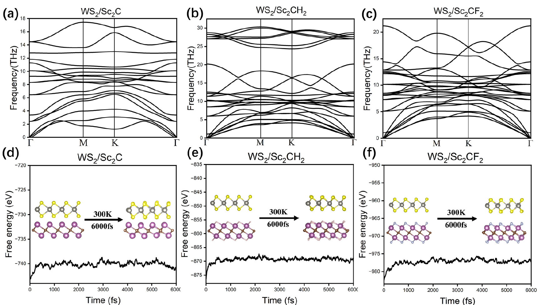
Bu 与 Sun 的 WS₂/Sc₂C 研究在 §2 说明 AIMD 使用 4×4×1 超胞,§3.1 给出 300 K、1 fs 步长和 6 ps 窗口。原文 PDF 第 5 页,Fig. 6(d–f)分别对应未修饰、H 修饰和 F 修饰的界面:横轴是 0–6000 fs,纵轴是各体系的能量(图上写为 Free energy,eV),黑色能量线旁同时放入初态、末态的侧视结构。各面板含不同组成,不能比较其绝对纵坐标高低来排列稳定性;作者依据各自时间序列与结构保持情况作分析,并将它们与上排 Fig. 6(a–c) 的沿高对称路径声子频率(THz)并列。
这类图应同时给出“何时采样”和“结构怎样变”。用现有 Al 数据复现时间序列时,读 thermo.csv 的温度与能量采样时间;查看初末结构时,先从扩展 XYZ 保留晶胞导出 POSCAR,再在 VESTA 中打开。已有 共同初态、粗步长末帧和细步长末帧;两份末帧都对应坐标时刻 48.37768653 fs。保持相同的视角、原子大小和放大比例比较,不能因为逐图缩放而把小位移看成明显重构。能量终点使用上面独立的采样时间,不把结构帧时刻直接贴到能量样本上。对真正的异质层,还应在对应结构图旁给出已有轨迹算出的层间距、侧向滑移或键长变化,而不只摆两张截图;本例 Al 记录没有层间统计,因此这些量接回 异质结构建模的层归属与法向定义。文献的 6 ps 是所用窗口,不能替代本例更短轨迹的实际范围。
这三份结构可在 al 根目录用 完整导出脚本复现:
python3 export_aimd_frames.py
脚本使用 ASE 读取扩展 XYZ 的 Lattice、周期边界和坐标时刻,输出到 nve-frames。它核对共同初态、八个 Al 原子、固定晶胞与末帧时刻,并读回 POSCAR 检查坐标未变;仅转换已有帧,不重新推进动力学。
导出环境需要 ASE 和 NumPy。要让编程助手写这一步,可以先给出下面的文件和核对要求:
用 ASE 读取两条 Al NVE 轨迹的扩展 XYZ,保存粗步长初帧和两条轨迹的末帧为 VASP5 POSCAR。保留八个 Al 的原子顺序、完整 Lattice、周期边界和坐标。核对两条初态一致、晶胞固定、末帧坐标时刻为 48.37768653 fs;写出后重新读入 POSCAR,比较晶胞与笛卡尔坐标。打印每帧原有的坐标时刻,让它和热力学表的能量采样时间分开记录。
export_aimd_frames.py 完整源码
"""Export existing Al NVE frames with their full periodic cells."""
from pathlib import Path
import sys
import numpy as np
from ase.io import read, write

root = Path(sys.argv[1]) if len(sys.argv) > 1 else Path(".")
out = Path(sys.argv[2]) if len(sys.argv) > 2 else Path("nve-frames")
out.mkdir(parents=True, exist_ok=True)
coarse = root / "aimd/nve-dt20-nosym/trajectory.xyz"
fine = root / "aimd/nve-dt10-nosym/trajectory.xyz"
initial = read(coarse, index=0, format="extxyz")
initial_fine = read(fine, index=0, format="extxyz")
assert np.allclose(initial.positions, initial_fine.positions, atol=1e-10, rtol=0)
assert np.allclose(initial.cell, initial_fine.cell, atol=1e-10, rtol=0)
frames = [("initial.POSCAR", initial),
          ("nve-dt20-end.POSCAR", read(coarse, index=-1, format="extxyz")),
          ("nve-dt10-end.POSCAR", read(fine, index=-1, format="extxyz"))]
for name, atoms in frames:
    assert len(atoms) == 8 and atoms.get_chemical_symbols() == ["Al"] * 8
    assert atoms.pbc.all() and np.allclose(atoms.cell, initial.cell, atol=1e-10, rtol=0)
    if name != "initial.POSCAR":
        assert abs(float(atoms.info["time_fs"]) - 48.37768653) < 1e-8
    path = out / name
    write(path, atoms, format="vasp", direct=True, vasp5=True, sort=False)
    restored = read(path, format="vasp")
    assert np.allclose(restored.cell, atoms.cell, atol=1e-10, rtol=0)
    assert np.allclose(restored.positions, atoms.positions, atol=1e-10, rtol=0)
    print(name, "coordinate_time_fs =", atoms.info["time_fs"])
原文把该 AIMD 图描述为自由能涨落;本例 QE 数据明确是程序打印的电子能量、离子动能与温度,不把单条轨迹的能量序列重新命名为材料自由能。要讨论温度下的界面稳定性,需用该材料实际轨迹说明采样期间观察到的结构变化,并把未出现的事件限制在所用超胞、温度和观察窗口内。